When a cave is surveyed, the survey needs to be fixed to a location on the surface at some point. This allows surveys of separate caves to be drawn together, and provides the coordinates of the entrance which can be supplied or shown on a map, so that visitors can find the cave. It also makes it possible for the cave to be studied in relation to the local geology or other nearby caves; which has the most easterly sink, the potential to connect to another, the greatest depth potential, or the oldest developmental levels?
The points in this article could equally apply to other fields such as archaeology, paleontology or biological/zoological habitat research, where mapping of remote sites is required. But caves have the particular restriction of needing most measurements to be performed in a place with no view of the sky, and without any standard maps aready in existence. As a result, a cave survey generally needs only a small number of surface fixes to tie to the centreline.
Typically, low quality cave surveys are located by looking for the approximate location on a map, and using that. Or alternatively, surveying from the nearest visible landmark on the map, which is located using the map. This can be highly inaccurate, as maps are generally approximated to make sure there is space for all the symbols, and they are not normally in high enough resolution.
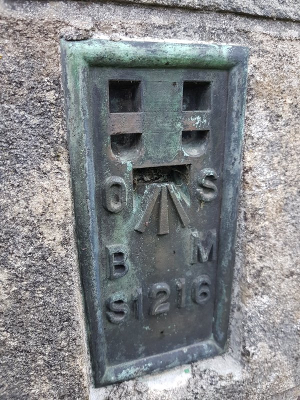
A better quality survey might require finding the nearest Ordnance Survey (OS) benchmark or OS trigpoint that still exists, and surveying all the way from that point. OS provide locations for these benchmarks to very high accuracy for altitude, but their horizontal positions can be given only to 10 or 100 metre precision, as their purpose was for surveying altitude, not position. That gives you a substantial error in the survey before you even start. Trigpoints have their positions given much more accurately (down to 1 mm precision, but with a 10 cm RMS error over the whole network) because their original purpose was as triangulation points for the horizontal positioning system, and in most cases also have a benchmark on them with a very precise height. Surveying from there will incur an error according to your survey's loop closure error (1% at grade 5), so a 1 km survey at grade 5 can have an error of ±10 metres, when surveyed to its expected accuracy. This adds to the benchmark location error. Unless you are very close to a benchmark with an official 10 figure grid reference, the chances are that the error is too high to be acceptable. Nevertheless, major surveys were traditionally located that way; the Mynydd Llangattwg caves were located in the 1950s using two trigpoints 5.7 km apart, with the caves linked by an extensive surface survey, with 3 km or more of survey linking a cave to a trigpoint. If you are able to use a trigpoint, use the most recent location provided by the OS database. Ordnance Survey have also fixed the points of a lot of random objects (bolts, rivets, belfries, chimneys, buried blocks, etc.) within towns, if you can somehow locate them, but in countryside areas where the caves are, trigpoints and benchmarks are usually the only options.
The positions of trigpoints, benchmarks and other features were all calculated using old surveying techniques, typically around 1950-1990, with many being at the older end of the scale. While the triangulation used to survey them has extremely impressive accuracy over such long distances, almost none have been resurveyed with modern approaches, and the specific errors of each of them is not known, though the standard deviation can be calculated by measuring distances from the primary network. A secondary (not the primary triangulation network) trigpoint in South Wales was measured as having a horizontal and vertical error of 3.6 cm each, for a total error of 5.1 cm. Horizontal errors get worse with each lower grade of triangulation (second order trigpoints can have a 6 cm error per 15 km from a first order trigpoint, for example), and with distance from western London (around 200 km in this case). Vertical errors get worse with each lower grade of levelling, and with increased over-land distance from Cornwall (around 375 km in this case). In this particular case, the expected vertical error margin given by Ordnance Survey is ±3.9 cm, which turned out to be quite an accurate prediction. The errors are just 0.000018% horizontal and 0.0000096% vertical, something a cave surveyor can only dream of. The same agency had measured the length of Great Britain between 1791 and 1853 with an error of just 0.002%, with triangulation based on a single 8 km length measured with glass rods and chains in 1784, as part of the Anglo-French Survey. Traditional surveying techniques are definitely impressive.
Satellite imagery may be used on maps or tools like Google Earth, to find an approximate location and altitude. This is often highly inaccurate, especially in mountainous areas. The satellite images are almost always taken on an angle, warping everything due to the sloping ground and perspective. This is combined with LIDAR scans which give an approximate terrain map (these are also very inaccurate, and can be worse in areas with trees), and the images are stretched back around the terrain, hoping to undo all of the warping. In bad cases, a point can move 30 metres or more in satellite images from different years. On top of that, for reasons given below, the actual location of the land being photographed is not known perfectly, because it is also located using the inaccuracies of the positioning systems. The end result is often fairly close in flat areas (perhaps 2-20 metres out) but the error can be extreme in mountains, sometimes tens of metres horizontally, and potentially hundreds vertically when cliffs are involved. The altitude is always an approximation, relating to an estimated sea level or earth model (typically a geoid model such as EGM96), not the local mapping altitude, and then applied to a LIDAR scan which might be at a resolution of only one reading every 15 metres horizontally (a gorge or shakehole can go missing completely). Trees can completely block the scans, hiding a 30 metre drop below them. Basically, this is such an inaccurate approach that it should not be used for cave surveying.
Most surveys are now fixed using a GPS (actually GNSS) device, though it is worth noting that these need to be used carefully to avoid significant errors. If they are recently switched on, and have not yet had time to contact enough satellites for a good location fix, the error can be 25 metres or more, though this improves when the device is given time to contact more. The same can happen if you only just stopped moving, and the device is using motion prediction. Under trees or near cliffs or buildings, they are as much as 5 times worse. The vertical error can be 2.5 times as high as the horizontal one; for vertical position, GPS devices can only see satellites for the half circle above the horizon, while for horizontal position they can see satellites positioned in a full circle around them. Industrial grade devices may be able to reduce the vertical error to around 1.7 times as high as the horizontal error. Most GPS devices give their accuracy predictions for horizontal only, because it looks better. With a basic phone GPS, 10-15 metres is about as good as you can hope for. Many devices are only designed to help you work out what road you are on, so they may even snap to the nearest road; high accuracy is not needed for that. The GPS feature of most phones is designed primarily to be used while moving, so they often have heavily damped positioning outputs which give incorrectly modified results. With advanced phones and dedicated handheld GPS devices, 6-10 metres is extremely good, but many seem to make very poor choices that cause them to give consistently bad results, with a 10-20 metre error being common. However, there are ways to get better results from a GPS device.
Bear in mind that most devices make exaggerated claims about how accurate they are. They may state an estimate of "2 m" (sometimes written with a ± symbol), but what they really mean is 2 metres CEP, or in other words; if you take 100 readings now, half of them will probably be within a 2 metre radius circle, but the other half will be outside it (the altitude is much worse). A much more honest result is called "2DRMS", which is a confidence of just over 95% (2 standard deviations) that the point lies within that radius. R95 is a confidence of 95%, so it is almost the same as 2DRMS. Most GPS devices use CEP rather than 2DRMS, because it looks better. If yours doesn't say, assume it is using CEP, and you should multiply by 1.2011 (GPS typically gets normal distribution in open terrain, so this factor usually works) to get a standard deviation or RMS, or 2.4022 to get 2DRMS. That "2 m" estimate is really 5 metres horizontally, and the vertical will still be much worse. This also means that you cannot directly compare the accuracy estimations claimed by devices, because they might be using different measurements. Professional grade devices, such as those made by Leica Geosystems, Carlson, Trimble and Topcon, or the Juniper Geode, usually use RMS, which is equivalent to a standard deviation, not CEP.
It is also worth noting that these estimates are not normally given from actual analysis of recordings (except in the case of land surveying base stations), and instead are an Estimated Position Error (EPE). This is a guess based on how many satellites are visible at which angles, ignoring reflections and ionospheric fluctuations. They are not a statement of the true accuracy of the readings.
A poorly designed GPS device might truncate precision enough to cause several more metres of error, might use approximated conversion routines that add a few metres of error, and might show completely false or modified altitude readings. Several popular devices make all these mistakes at the same time. These errors are hard to detect, as the device can make the same mistake every time you use it, so it looks like the results are good. The results can be extremely good at one spot where you are testing, while the mistakes all cause issues elsewhere. In general, a handheld GPS that you might use for navigation in the mountains, should not be trusted for surveying. The rest of this article will cover what to watch out for, and how to get good results from a GPS device.
If you are surveying only a single cave, and there is no chance that cave could ever connect to another cave, then the accuracy of the fixed location is not really important. But once two caves are involved, it becomes much more significant. If the surveys of two caves are fixed only approximately, it is possible that the two caves could appear to intersect in places that they do not intersect. Depending on how poorly the entrances are located, they could appear to be on the wrong side of each other, such that the cave on the left is shown as being on the right in the surveys when they are drawn together. Vertical accuracy is also very significant when a sink and resurgence cave are surveyed separately, or when trying to work out how much more depth might be obtained before reaching the water table. The water might be last seen flowing down a hole in the floor of the sink cave at a lower height than where it is first seen in the resurgence cave; an impossible situation. This makes it very difficult to combine the two surveys in a meaningful way, and it makes study of the caves challenging, both from a digging and scientific perspective.
One approach to avoiding this would be to fix all cave surveys in an entire catchment to the same location - a rock, trigpoint, fencepost or any other fixed feature - so that no matter how badly the initial fix was made, every survey will share the same error (in addition to their individual surface survey errors). This works until someone else chooses to survey a different cave in the same area without knowing about the special place they were supposed to have started, 2 km further down the valley, so they fix it using some other location. Nevertheless, this approach is used in some areas, ignoring how badly it will fail in the future.
When two caves that connect are surveyed from separate fixed locations, if there is a very significant error in the location fixes, then the error needs to be distributed throughout the surveys, causing substantial distortion of the survey, and a degrading of the survey in terms of its loop closure. Ideally, a location fix should be done as accurately as possible, so that it does not degrade the quality of the surveyed centreline, in such cases. If you can only fix a location to 3 metres accuracy horizontally and 8 metres vertically (which is actually very good for a consumer grade GPS), then rather than fixing 2 entrances separately, it is actually better to survey over land for over 1600 metres to get from one entrance to another at grade 5, or over 8 km if you are surveying with a Disto! Having a way to locate entrances as accurately as you can survey between them, can save you a huge amount of surface surveying.
GPS was the first satellite based navigation system made available for public use (1980), and the name stuck. However, there are several systems available, some covering the whole globe (like GPS) and some covering just one country or continent. The big ones are USA's global GPS, Europe's global Galileo, Russia's global GLONASS, China's global BeiDou/COMPASS/BDS and India's IRNSS/NavIC. Japan is still developing QZSS. IRNSS/NavIC covers an area from southeastern Europe and eastern Africa to China and Australia using geostationary satellites. QZSS covers only the area between Japan and Australia with geosynchronous satellites. The collection of satellites from each system is known as a constellation. Collectively these are called GNSS or RNSS systems, and anything that uses these systems is called a GNSS device, also known as a receiver or rover. Most "GPS" devices are actually GNSS devices, and can use whatever satellites are available to them, not just the GPS satellites. If they can use more than one constellation at once, they are called multi-GNSS, but can also be stated as dual-band or multi-band, which confuses it with multiple frequency. This allows them to see more satellites at once, and therefore give better accuracy in conditions where obstructions might block the view of some satellites.
Historically, the USA GPS system used to intentionally give incorrect results of up to 100 metres, for defence purposes (the Chinese national mapping system still plays similar games within China), known as Selective Availability. This affected readings everywhere in the World. The USA stopped doing that in 2000, but the USA GPS system is still one of the poorest of the major systems. Many areas of the world still randomly see very poor GPS results because of it, while others such as Europe have far better systems, as well as systems designed to - at least partially - correct the mistakes of the GPS system. GPS is not bad, but it is out of date, and it needs assistance to compete with the results of the other systems. All of these systems are able to give better features or accuracy for military usage, with public services in some of them limited to less accuracy.
Most of these systems work in the same way; the satellites send out a message giving their position and the time on their highly accurate clock (actually they give out a lot more than that, including information to help devices to locate other satellites). The GNSS device checks for the differences between those clocks, to work out how far away each satellite is. The exception is BeiDou, which can use two-way communication if the GNSS device supports it, letting the satellites know where the GNSS device is (which could be considered a privacy risk) - that feature seems to be part of their high accuracy mode, and is not used by normal consumer devices.
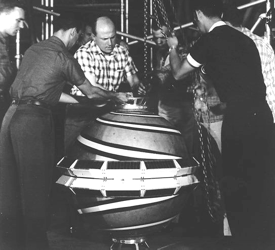
Historically, the first system was the US Navy's NNSS/Transit, which worked in a completely different way, using the Doppler effect. It required very careful analysis over a timespan of about 2 minutes, to give a final accuracy of around 100 metres. The Soviet Union had their own Tsiklon system using the same idea, which needed 5-15 minutes of monitoring a signal to calculate a position to 100 metres accuracy, within intermittent time slots. Neither of these systems are in use any more, and they are not compatible with the current GNSS systems.
There are different ways that devices may choose to use the different constellations. They may use the satellites at the same time as if they were one constellation (and this is essentially what most GNSS devices will do). They may use each constellation separately and get an average of the positions given by each of them. Or they may be able to use the results of one constellation to calculate the likely errors of another constellation, and correct the position based on that.
There are several ways to improve GNSS accuracy. The main ones are GPS/GNSS averaging, multi-GNSS (covered above), differential or relative GPS/GNSS, satellite augmentation, dual or multiple frequency, carrier phase tracking, doppler, real-time precise point positioning and post-processing. There are also some factors in how to set up and use a device.
There are several causes of error in GNSS readings that have varying impacts, and each of the ways to obtain better accuracy might only be trying to reduce a few of them. The main causes of errors are: dilution of precision (1-20 times the device's expected accuracy), signal obstructions (normally ±25 metres horizontally in severe cases), ionosphere delays (±5 metres horizontally), alignment of the coarse satellite messages (±3 metres horizontally), satellite orbit errors (±2.5 metres horizontally), satellite clock errors (±2 metres horizontally), reflections and multipath (±1-5 metres), mathematical limitations of the device (±1 metre horizontally), troposphere delay (±0.5 metres horizontally), and alignment of the precise satellite messages (± 0.3 metres horizontally).
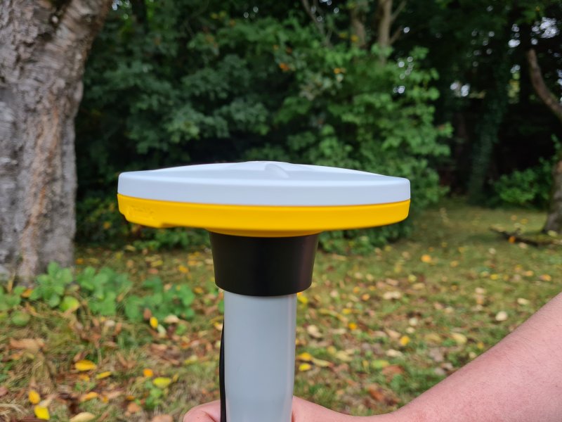
Some devices may need to be positioned antenna (aerial) upwards if the antenna points out of the top of the device. A CT8 (described below) should lie flat, the location of its antenna is shown on the back of the case. Most high quality antennae will need to be oriented pointing upwards if they are long and thin, or with a flat, circular antenna, they should usually be oriented with the circle oriented horizontally.
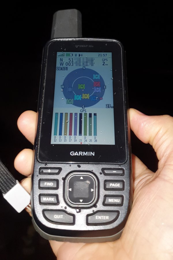
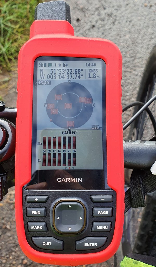
High quality antennae will tell you the reference point where the measurements are relative to, often slightly above the antenna for a simple antenna, or the base of the antenna for a device that has all of the computational electronics inside it. If it does not tell you, the location fix will be somewhere close to the location of the antenna (but not actually touching it) in most cases. With a phone, this is often somewhere near the top corner on the opposite side from the camera, and typically functions best with the screen facing upwards. With a handheld device that has a helical antenna (such as a Garmin GPSMAP 66sr), this is usually inside the middle of the antenna, and either about 40% of the way up the antenna, or at the base of the antenna, depending on whether the device intentionally subtracts an offset to give the location of the base.
Blocking of the signal is an important consideration. Tall buildings or other obstructions block signals or add reflections (multipath), and reduce accuracy or create a bias. Reflected signals have taken a longer route to reach the device than they would have done if they travelled directly from a satellite, so the device can think it is further from the satellite than it really is. Buildings might not be such a problem for caves, but cliffs, trees and reflective surfaces like lakes certainly are. If your device relies on satellite augmentation (SBAS) for accuracy, then a clear view will be needed towards those satellites - in Europe, they sit above the southern horizon. If your device relies on correctional data being sent from a base station, then the corrections can become useless when there is too much tree cover, as the device and base station often cannot see enough of the same satellites as each other.
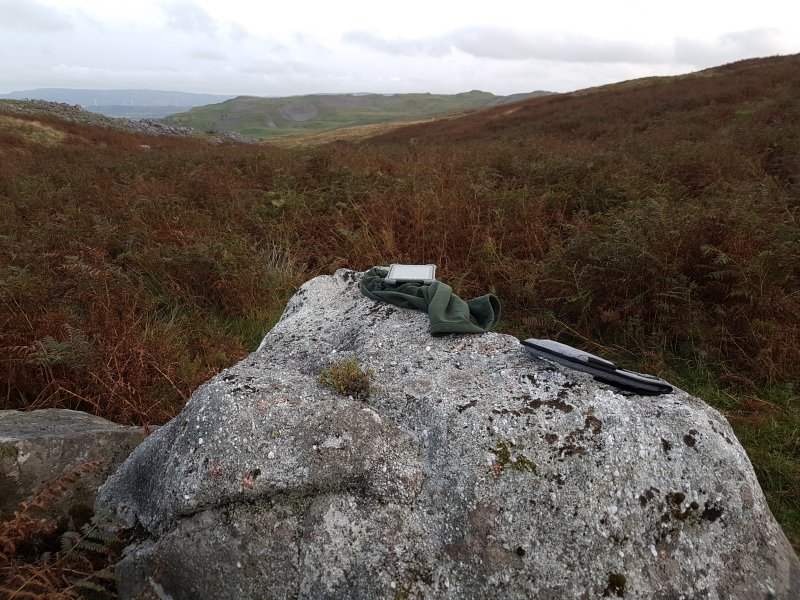
If at all possible, fixing a location should be done away from buildings, cars, cliffs, trees and lakes to get the best results - it is better to survey in from a place with a good location fix. Ideally, the device (or its antenna) should be elevated off the ground by a fixed distance of at least a metre or two, such as on a tripod or tall object, to avoid low lying obstacles and bumps from blocking signals - higher is better. A fencepost in a field is a much better choice than the bottom of a shakehole. A rock pinnacle is better than the side of a cliff. A location fix in a forest should only be considered if there is nowhere nearby to get a better location accuracy. If you can survey in from the nearest open space with an error of 1 metre, that is better than losing 2 metres of accuracy below trees. This will all depend on the quality of your device, but even high quality devices lose some level of accuracy below trees. An external antenna can improve signals for some devices or in difficult areas, if the device allows it. When you stand above your device, you will block most of the signal, so for the most part, the device should be left alone while it is recording; this is not an issue if it is mounted above head height.
With devices that have poor handling of multipath signals, it can also help to put an earthed metal plate below the device, to catch any signals that are being reflected upwards towards the device. An earthed choke ring (several rings of metal fins) - like those seen on a professional grade antenna - works far better, but if you can afford one of those, buy a proper GNSS antenna. It is worth noting that handheld devices are typically designed to record GNSS data even when lying at the wrong angle in a backpack, and phones are designed to pick up signals even when strapped upside down in a holster or pocket. These devices intentionally pick up signals from any angle, and that causes them to detect large amounts of multipath signals reflected off the ground or nearby objects.
After switching on the GNSS device or its GNSS chip, it can take a long time for the best accuracy to be achieved. If a device has not been used for a while, or has dramatically changed position since it was last used (and any existing almanac data has therefore expired or become irrelevant), it must start by scanning for satellites. This is known as a cold start. Once it has detected one, it can use almanac data from that satellite to find the others faster, and hopefully find enough to get a location fix. This can take up to 13 minutes. The reason for this is that the satelites send out a long message containing the locations of the others in their constellation (rough almanac data), over the course of 12.5 minutes. The device can use that to narrow down its scanning to locate the subsequent satellites. Each satellite then sends out its more accurate position information (ephemeris) every 30 seconds. If the GNSS device was recently used, and has valid almanac or ephemeris information, it can skip the 12.5 minute cycle, but still needs to find the satellites that it expects to be able to see, and check that the right frequencies are available. The device can also continue to scan for satellites without having Almanac data, but that can take a long time, depending on the device. Almanac data is valid for 90 or 180 days, while ephemeris data is valid only for 4 hours. Starting up the device the day before you plan to use it, and running it for half an hour so that it can locate almanac data, is a good idea; the next day, it can perform a warm start instead of a cold start. If it is started within 4 hours of the time it will be used, so that it still has valid ephemeris data, it can perform a hot start instead.
Once the device has located the satellites, it can then start using their signals to work out its location (the delays up until this point are known as the Time To First Fix, TTFF). As the device locks onto more and more satellites, it can refine its position more and more to reach its highest accuracy level. With a Juniper Cedar CT8, for example, this usually takes about 1 minute after its initial location fix. Some devices will take a couple of minutes, or longer when the signal is obstructed. With higher accuracy devices, such as those using RTPPP, this can take a lot longer to get beyond a basic fix, and down to the centimetre or millimetre level accuracy (this can be much faster with NRTK devices). Half an hour is not impossible. Check how long your device typically takes, and be willing to wait that long before taking readings. If it is taking a long time to reach the expected accuracy, wait for longer and see if the situation improves.
The device needs to be static; readings must not be taken while in motion. Motion causes the signals from different satellites to be received in slightly different positions from each other, which can really confuse the resulting calculated position. A device might also think it needs to guess where it is, if the position is requested in between position fixes. Many devices employ motion prediction if they think the device is moving, so the resulting position is an estimate, not a real measure. If a device has just stopped moving, then it needs to be kept still enough for motion prediction to have stopped being used. This varies with the device, but most devices should be given a minute or more at rest before taking readings. While a device is initially refining its position, it might think it is moving even when it is staying still. Some devices allow you to disable motion prediction. On Android devices, such as the Juniper Cedar CT8, the location settings may have an option to set the positioning to be set into "static" mode, so that they do not try to use motion prediction in between readings.
Some devices - particularly those designed to record cycling or jogging - will also smooth out any jitters in position, which they assume is an error, even if it is actually a real movement. Basically, they give results that they have modified or falsified. Some allow you to disable motion smoothing. In general, devices with built-in motion smoothing will use it because of how poor their GNSS results are, so they are best avoided anyway.
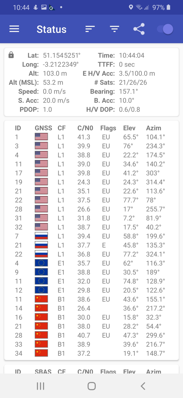
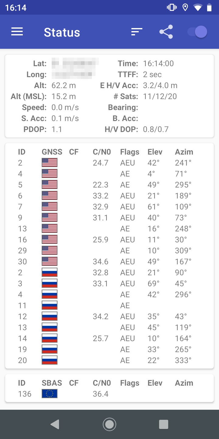
For Android devices, the GPSTest app from barbeauDev can be used to see what level of accuracy has currently been reached, and whether the readings appear to have stabilised. For a Juniper Cedar CT8, this is usually less than 1 metre, perhaps 80-90 cm. (Note; do not leave the app running while taking readings using a different app, because it uses a lot of battery.)
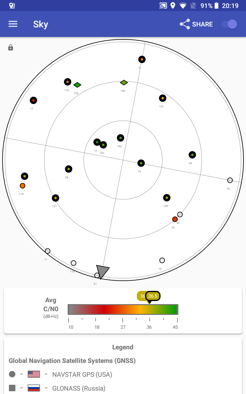
GNSS satellites constantly move. There are times when there are lots above you, and times when there are fewer. A GNSS device normally needs 4 to get a location fix (knowing how far each of them are from you, and where the spheres at that radius from the satellites intersect), but it helps to have more. If all 4 are directly above you, they will be able to work out your altitude fairly well, but not your horizontal position. If all 4 are near the horizon, they will be unable to work out your altitude, and there will be more refraction and distortion of the signals from the ionosphere, so the horizontal and vertical results will be randomly skewed. If all 4 are in the same direction from you or spread out in a line, they cannot triangulate your position well. The best results are when there are at least 4 satellites at roughly 45° above you, spread out in a circle. This is all known as dilution of precision (DOP).
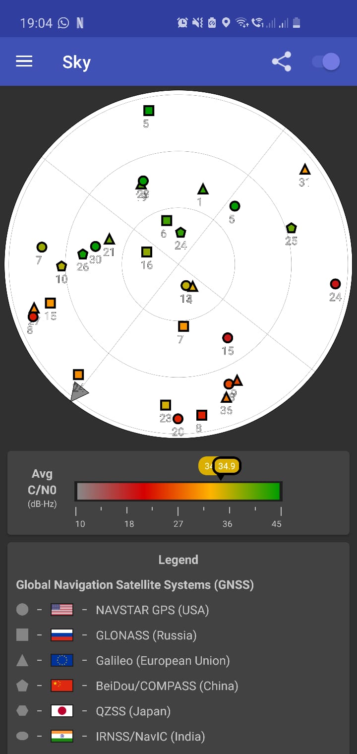
Modern devices can see satellites from multiple constellations, and in general, there are almost always enough satellites above you for the device to use perhaps 10 for a location fix, with enough being at a good angle. To plan the best times for readings, you will need to know which satellite constellations your device uses at any given moment. For Android devices, use the GPSTest app from barbeauDev to check what satellites your device can see when you stand outside. For other devices, they might have a similar function showing a satellite map with constellation names, or it might be in their documentation.
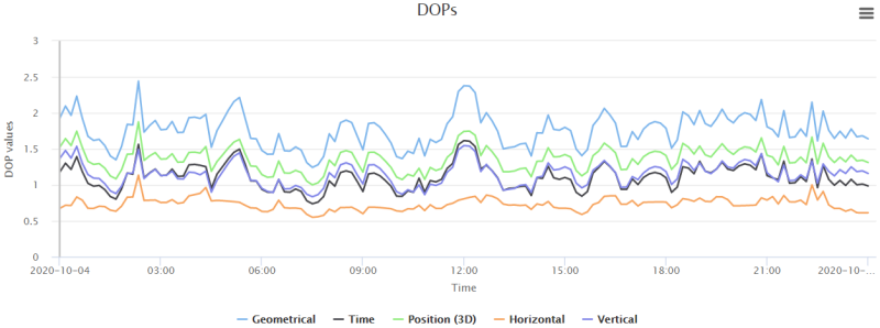
Once you know which constellations your device sees, you can use the Trimble GNSS planning tool to see when the satellites will be good for taking readings. On the settings tab, set the constellations, approximate location (use your favourite online mapping tool to get the approximate coordinates and height). Then fill in the date that you hope to take readings, and select the full 24 hour view for that date. Apply it, then view the Charts tab. Scroll to the "DOPs" chart, and see if it has any big spikes on it. For best results, you want to take readings at times when it is as steady as possible, ideally remaining below 2.5, and definitely remaining below 5.
The ionosphere also plays a big part. The ionosphere fluctuates constantly, creating small distortions in the satellite signals. In the depth of night, these effects are reduced. During the day, the heat from the sun causes more small ripples. The worst time of day is after dusk, when there is a big change from hot to cold, rolling around the earth for a couple of hours either side of your position. This can cause effects such as plasma bubbles, rising through the ionosphere, with the worst effects near the equator. Dual frequency devices are affected less, and devices with satellite augmentation are also affected less. The better your device, the more times of day you can rely on it, but even with a good device, it is best to avoid dusk.
The sun's 11 year solar cycle causes substantial distortions that can cause even the best GNSS devices to struggle. Avoid taking readings whenever there is a lot of solar activity - basically any time that the world is experiencing very strong auroras, or whenever there is a report on the news about degraded GPS/GNSS signals. There are lots of aurora prediction services around, but Trimble's GNSS planning tool also has a chart for Iono Information. You can also use many phone apps to predict aurora borealis (northern lights) activity, and avoid any time when the Kp-index is high enough to cause a lot of northern lights activity, or activity to extend down a long way from the poles.
Military and police can sometimes intentionally jam GNSS signals, or cause them to become severely distorted. It is also possible for this to be done for malicious purposes. When the military are testing this system, it is usually announced beforehand, and may appear on news sites.
Water droplets in the atmosphere do not affect the GNSS frequencies very much at all. As a result, storms and cloud cover have only a very small effect, though your GNSS device may not function when covered in ice, drowned in water, or hit by lightning. It is probably best to avoid fixing locations in those conditions, if you value your own safety.
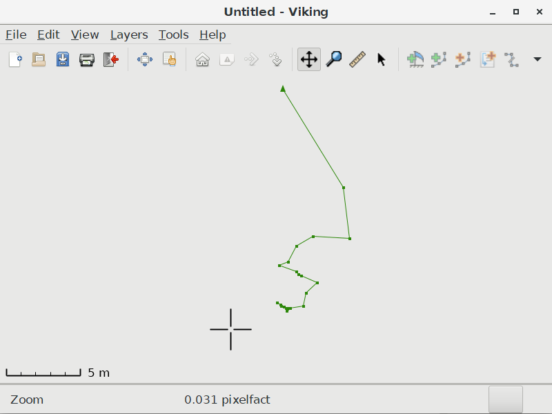
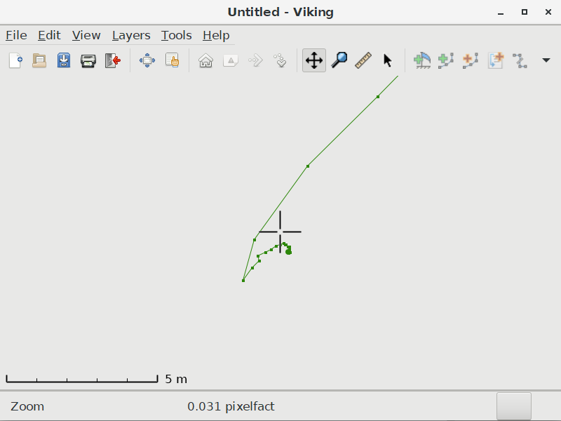
GPS positions vary over time, even when the device is staying still. Sometimes the position can be wildly out for a few minutes, then settle back to normal - meanwhile your device is still claiming "2 m" accuracy. Taking multiple readings over several hours or days, and averaging them, usually gives a much better refined location. It is even better if you can use something like a Kalman filter to concentrate on positions that are clustered together, and ignore the odd positions that are far from the main cluster. Doing this several times over several days and averaging those (preferably weighted averaging using standard deviation, something Survex and Therion can do for you), will help iron out daily variances in GNSS positioning. If you fix more than one point in the survey, supplying standard deviations for them and the survey between them will allow Survex and Therion to distribute the errors between all of them correctly, and calculate the overall positions.
Averaging cannot fix everything. If there are obstructions or signal reflections affecting an area, or if the available satellites offer a consistently incorrect position, the position can have a bias in one direction, so that even a long-term average can remain wrong.
Averaging cannot turn a low quality GNSS device into a good GNSS device, though it does help smooth out the large deviations between individual readings. Averaging for 3 hours with a Samsung Galaxy A40 saw the average position wander around by 3.5 metres, and the final position remained 3.5 metres horizontally and 10 metres vertically from the correct position, with a very heavy bias in one direction. At no point did it approach the correct location, and the vertical error remained consistently terrible. The data showed a very good standard deviation both with and without Kalman filtering, substantially smaller than the actual error. This shows that the standard deviation is largely meaningless with a poor GNSS device, as the bias can cause the position to be consistently wrong by more than that amount. The only way to know if your device is behaving poorly is to compare it with a known location, such as a trigpoint (preferably one with a similar number of obstructions to what you will have at the place you will be surveying - a clear view of the sky might not be realistic).
There is a question of how long to perform averaging. If your device takes about one reading per second, and has a stated accuracy of about 1 metre (a very good device), then a good plan is about 3 hours at a time, a couple of times in one day, perhaps repeated again on another day. But you should test your device several times on different days, and see how close each result was to the last one. When taking thousands of readings over the course of 3 hours, how much has the average changed after each hour? Ignore the standard deviation numbers for now. If the average is still wandering around in circles a few metres across, or the vertical change is several metres, you should average for longer. Try again another day, how do the results compare with last time?
Some devices offer GPS/GNSS averaging as a feature. This is common with handheld devices, for example. Some require you to manually press a button to obtain a new reading every few minutes; this is not particularly helpful, since you really want it to have hundreds or thousands of readings to average. For Android devices (assuming the device can actually give a real GPS positioning output), there are several apps that can do averaging, but most completely disregard the accuracy of each reading, and will give just as much priority to a 15 m accuracy reading as they do for a 2 m accuracy reading, so the results can be very poor. A single very poor reading can throw off the average for a long time, and several readings with a signifcant bias can cause the overall average to be unusable. Most averaging apps do not use any kind of filtering, and those that do generally do not allow you to control the type of filtering that they do use. Almost none allow you to see the standard deviation of the results, which is useful for Survex and Therion. Even fewer allow you to see the vertical standard deviation, which is important, since it is usually much worse than the horizontal. Currently, there do not appear to be any properly maintained apps for Android that can do Kalman filtered results, while also giving you the latitude, longitude and altitude standard deviations. Please get in touch if you discover one.
Although discontinued, Elec Otago Position Estimator is an app that offers all the important controls and information. It is no longer maintained, and cannot be downloaded from the Android Play store any more; it now has to be downloaded as an external APK. In the settings, the "Independent Kalman Filter" setting allows it to discard readings that were too far away from the normal, and allows it to take readings for longer without choking on the amount of data. The app allows you to see the standard deviation of all three coordinates separately. Note, however, that the standard deviation in most filtering modes is a faulty estimate based on how many samples it has taken, and what filtering it is using; it is not a real measure of the standard deviation. In testing with a device that gave 2-3 cm accuracy, the app continued to say that the standard deviation was over 5 metres, which is definitely not correct. Switching it into "Position Averaging Filter" mode allows you to see the real standard deviation of the results, rather than an estimate. This mode can be switched at any time, but be aware that it can crash on some devices if it has been gathering data for a long time, so it helps to pause it before switching. It is not possible to see accurate Kalman filtered standard deviations. (Note that the app always says it can see 0 satellites on most devices - that is a bug that can be ignored.) Position Estimator records altitudes at 1 cm precision, which is fine for most purposes. The app does not allow you to access the actual data that it has collected, you can only see the results.
When performing averaging, it is best to use an app that allows you to access the data that it has gathered. This will allow you to decide exactly what analysis to perform with the data, discard faulty readings, or operate only on a subset of the data. When using a high accuracy GNSS antenna or refining the position of a highly accurate GNSS device, you should ideally use an app that gathers readings at high precision; there is not much point in having a GNSS device that can record data at 10 cm accuracy, if the app can only recrd data at 1 m precision. For averaging (with or without Kalman filtering), you ideally want an app that records data at a far higher precision than your device's accuracy, since the jitters at that higher precision are what will be averaged to obtain the final location. Some GPS track recording apps can record data at high precision, so that you can view the data and manipulate it yourself in whatever computer application suits you. Almost all of these apps (including Locus Maps) truncate the data to a low precision that is worse than Position Estimator. However, a future update to the GPSTest app from barbeauDev, will make it possible to record logs in the full detail that comes from the GNSS device itself; in the settings, enable logging of location, and the data will be outputted in CSV format, saved into a file on the device. Usefully, the horizontal and vertical Estimated Position Error (EPE) will also be recorded for each reading, which allows it to be used for Kalman filtering. Google's GnssLogger can record similar data, but it does not record the vertical EPE, and caps the data precision to 7 decimal places, about 1 cm at best. The logs recorded with these apps can be processed using the HowToCreate GPS/GNSS log file parser, which outputs results with Kalman filtering, and gives separate standard deviations for latitude (northing), longitude (easting), altitude. This tool was developed specifically for use with locating cave surveys. GPSTest 4.0+ and the HowToCreate GPS/GNSS log file parser, are the recommended approach for averaging on Android.
For logging of more minimalistic data, an alternative app is GPX Recorder. It is an extremely basic app, which simply records GPX tracks and lets you export them, without truncating data. The GPX files it creates are fairly simple, and can be fairly easily manually converted into a more useful format using a text editor, such as a CSV which can be opened as a spreadsheet. It only initialises the GNSS after the recording starts, so the first few minutes of data may need to be removed from any averaging to allow the GNSS position to initially be refined. The EPE is not recorded.
If all you end up with is a log of all the readings, you will need to average the positions yourself. This can be done by loading the data into a spreadsheet (very easy if the app outputs in CSV format), then using the sum and average feature of the spreadsheet application. The latitude, longitude and altitude can be used to calculate the standard deviations of the northing, easting and height. Optionally, the EPE can be used for weighting the results if the app recorded it, but this requires more significant programming. Or alternatively, you could implement your own Kalman filtering on the results, but this requires even more programming (and at this stage, it is best to use the HowToCreate GPS/GNSS log file parser, since it is designed for this purpose).
Android has a few power considerations (aside from the possible need for an external battery pack). In the Android app permissions, you will need to ensure that the app is allowed to access the position even when running in the background, just in case some other app steals the focus. Keep the app focused anyway, just in case. In the Android app settings, ensure that Android does not optimise battery usage for that app (so it doesn't close it automatically when it thinks you are not using it). In the Android battery settings, ensure that it never puts that app to sleep. In personal testing, this continues to work even if the screen is switched off, but external USB antennae might be switched off, if you are using one. The Awaker app can keep your screen on if your device does not have a setting for it. Ideally, you should also tell Android 9+ not to sleep the GNSS chip randomly after a few seconds of use (known as duty cycling). Enable Developer options; in Android settings go to "About phone - Software information" and tap 7 times on "Build number". Go back to the settings page, then into "Developer options" and enable "Force full GNSS measurements".
When using Kalman filtering, it is very important to use static Kalman filtering, not dynamic/kinematic Kalman filtering. Static Kalman filtering uses all of the data, concentrating on the results with the best EPE, that are in the main cluster. This allows it to refine a position to incredibly high detail, using a large amount of data for a single point. Dynamic/kinematic Kalman filtering is designed to ignore older results, and concentrate on the most recent results, until the data changes too much. At that point, the older results get increasingly ignored again, and the new position is calculated; it is designed to smooth out the jitters in tracks created by a moving GNSS device. It is not designed to use a large amount of data to refine a single position.
Warning; many Android devices and all iPhones present false GNSS readings to apps. With Samsung Galaxy models (tested with the S7, S10, S20 and S21 series), the position updates initially for a while, then once the device has decided it is not moving, it stops updating the position, even if it is still far from the correct position; the altitude might continue updating for a while, but often that then stops updating too. Similar behaviour can be seen on iPhones and many other Android devices, where the coordinates change, but only after waiting for several seconds, and only by the tiniest amount, such as 1 mm or less, even though the position is still many metres away from the correct location. Small movements (eg. 30 cm) are often ignored by these devices. Only after the device has moved far enough away, or if the GNSS location has shifted far enough, will it start to update the position properly. This appears to be a type of kinematic (not static) Kalman filtering that is applied by the device's GNSS chip. While static Kalman filtering can help with averaging, it does not help when the device tries to apply kinematic Kalman filtering, since that simply causes it to present false readings to apps, whether it is being kept still or in motion. During testing, all of these devices stopped updating while the position was still several metres away from the correct position (the vertical errors were generally far beyond acceptable limits).
Needless to say, if your device tries to apply any movement damping, smoothing or kinematic Kalman filtering to the GNSS output, you must not use it for averaging, as it will only rarely bother to update the position; the statistics will look incredible, but the data it gathers is complete nonsense. iPhones cannot be made to behave correctly, and also have other issues that make them unusable for surveying, discussed below. Older Galaxy devices used to have a location setting where you could disable the built-in kinematic Kalman filtering, but this has disappeared on newer Galaxy models. You can test for this problem by putting the phone out in the open where it can get a reasonable location fix, such as on a wall. Look at the Status page in GPSTest (or the GPS Data app on iOS), and wait for it to get a location fix down to its normal accuracy (eg. "4 metres"). Real GPS positions change constantly. Keep the device very still. If the position shown by GPSTest slowly refines then stops updating within a minute or two, or shows only the last digit changing slowly, then your device cannot be used for averaging. A device with 1 metre accuracy still shows the 6th and 7th decimal place digits of the longitude and latitude updating every second or so (that is a roughly 10 cm wobble every second). Unless your device can actually do 1 cm accuracy, you should be seeing those numbers change! In general, this makes most phones unusable for this purpose, even if they have many other advanced GNSS features. They are designed for helping you navigate along a street or path while moving, and they are not intended to be used for surveying. A phone should only be considered if it either does not exhibit this behaviour, or if it allows the behaviour to be disabled in its location settings. When using an external GNSS antenna, this problem generally does not occur, since it is caused by the firmware that controls the built-in GNSS chip. As a result, external antennae can make a phone usable again.

A differential or relative GPS/GNSS system uses one or more fixed GNSS stations, to monitor satellite signals and provide corrections in realtime for devices that are using GNSS near that location. This may be a base station where you have worked out the exact position yourself, sending Real-Time Kinematic (RTK) corrections to your GNSS device over a network cable or radio link. More commonly, however, it is a very expensive system where you use someone else's base stations located around the country over the Internet to send you corrections (using protocols such as NTRIP). These base stations are known as Continuously Operating Reference Stations (CORS). It has the major advantage that if the GNSS device is positioned between multiple base stations, it can use correctional data from several at once, calculating the most likely signal distortions affecting its own area, and also getting details of satellites that can only be seen by a minority of the stations. This is known as Networked RTK (NRTK), and allows the CORS network to have bigger gaps between stations. There is also Long Baseline RTK (LBRTK), which is where the probable ionospheric distortion and satellite orbital corrections are modelled far away from from a base station, and delivered along with the RTK data from that single base station. This allows it to work at much greater distances, and is used by national base stations in some countries (such as Turkey). The good part with any of these (N)RTK systems is that you can just take a single reading and have a highly accurate location fix for your survey. NRTK is able to obtain the highest accuracy level of any realtime GNSS approach, and RTK/NRTK is normally also the fastest high accuracy method to initialise.
In all cases, a GNSS device that uses a base station may also be known as a "rover". The rover needs to authenticate and work out which base stations to use (in cases where multiple are available), and this requires a two-way network communication. The correctional data can augment only the standard satellite "code" messages (in which case it is typically known as DGPS or DGNSS), or it can also correct the carrier phase too (at which point it gets known as RTK or NRTK). Code phase based DGPS/DGNSS can normally give results accurate to about 30 cm horizontally; it was the first differential GNSS approach to be developed, and is now used mainly in devices that offer a lower priced low-precision option. Carrier phase corrections allow a device to be far more accurate, but require higher bandwidth, 5-10 kbps depending on how many constellations and frequencies are used. Carrier phase tracking will be discussed further below.
The base station simply records what it sees, and sends its true position and the observations it has made, to either the GNSS device or a control centre, which can work out how far wrong each satellite's message appears to be; this is known as Observation Space Representation (OSR). It compensates for delays or incorrect timings in the satellite signals, satellite positioning errors, and ionospheric and tropospheric distortion all at once. It does not compensate for reflections/multipath or mistakes made by the GNSS device. For this to be useful, the base station needs to see the same satellites as the rover, and the same signal distortions. 25-35 km is best for a single base station, but NRTK systems manage to do well in the 70-100 km range, and Long Baseline RTK can work at even greater distances. In theory, NRTK allows the device to simply receive all data for all stations, removing the need for two-way communication, but the amount of data becomes substantially higher, so a high bandwidth connection would then be needed. As a result, NRTK usually relies on a control centre to collect the data, and send only the appropriate parts to the device over the Internet.
Some GNSS devices can also use free RTK base stations. There are 7 high quality ones within the UK which require registration, and several privately operated ones located around the World which can be used as long as they are reliabily available and support the right constelations. (There are many more in France.) The low number of sources means that corrections being sent to your device might be from a station 300 km away, which sees different satellites and somewhat different GNSS signal distortions, and accuracy will be limited by that (a high quality device might be able to get about 30 cm accuracy when using a base station at that distance in ideal conditions). The base stations can also be incorrectly located; it is rare for free base stations to advertise how accurately they are positioned or calibrated, or which reference frame and epoch their positions are given in; some may use WGS84 positions for whichever date they were set up in, while others will be in a local reference frame, such as one of the ETRS89 frames in Europe.
If the base station and rover cannot see enough of the same satellites, then the result may be called "RTK float", meaning that the rover is largely acting like a basic GNSS device, with only a few satellites having RTK data; the result is similar to not using RTK. It will work best when at least 5 satellites can be seen both by the base station and rover, at which point it is called "RTK fixed". If the base station and rover cannot see enough of the same satellites for even "RTK float" quality fixes, then the rover will typically revert to being a basic GNSS device, perhaps with SBAS, if it supports that. As a result, working in areas with overhead trees is almost impossible, even with a good NRTK device, and location fixes will still need to be done in areas with a good view of the sky.
It is important to note that when talking about RTK or NRTK, the accuracy shown on the GNSS device is the relative accuracy. It may say that it has an accuracy of 1 cm RMS, but that is an accuracy relative to the base station. For example, a poorly configured base station could have an error of ±1 metre RMS. That means that the GNSS device has an absolute accuracy of ±1 metre ±1 cm (so ±1.01 metres total) RMS. When using the OS Net base stations (CORS) within Great Britain, the base stations are considered to have no error, because they are the fundamental base stations of the British mapping system. When using any other base stations, the base station could have its own inaccuracies when compared against OS Net. An NRTK device that can directly use the OS Net base stations (or national equivalents elsewhere) is therefore the most desirable. (The actual error of the OS Net base stations was measured in 2006 as 11 mm easting, 16 mm northing and 31 mm height RMS, but there has been a big upgrade since then. The current equipment has a standard error of 8 mm horizontally and 20 mm vertically - presumed to be a standard deviation.)
In 2020, one of the lower cost differential GNSS devices is the Juniper Geode, which has an impressive accuracy of ±25-30 cm (60 cm 2DRMS) even without enabling RTK, and retails for around £2000. You can improve its accuracy to around 10 cm by enabling it to use free RTK sources. There are also much lower cost ArduSimple systems available, which retail for around £380 (note that helical antenna designs pick up a lot more reflections, and are not recommended). These devices generally rely completely on free RTK, and therefore need a network connection. Their accuracy without a network connection (such as in the mountains, where caves tend to be) is similar to a basic GNSS device. Their stated accuracy of just 1 cm depends on there being a base station within 35 km that corrects the right constellations and frequencies. In personal testing, using a base station 100 km away allowed the device to obtain a horizontal accuracy of 2.9 cm and vertical accuracy of 4 cm, which was much better than the 1 cm + 1 ppm formula predicted. ArduSimple accuracy is stated in CEP, not RMS, and the results were therefore spread over the expected 10.5 cm radius circle. In personal testing, the vertical position occasionally jumped 90 cm away from the correct position, significantly further than the expected 15 cm; this could have been due to a loss of RTK correction data. The ArduSimple device, when used via a Bluetooth connection with the Lefebure app on Android, occasionally dropped out for a second or so, causing Android to revert to the inbuilt GNSS antenna during that time. This caused issues when averaging or taking single readings.
Higher quality NRTK systems may be able to give you a location fix down to 1-2 cm anywhere in the country but usually cost £5000-25000, and NRTK subscriptions are usually over £1200 per year. The better quality ones have more NRTK base stations (CORS), so the corrections are specific to your location. The main high precision NRTK services in Great Britain are Ordnance Survey's OS Net which uses about 115 base stations, Leica/HxGN SmartNet which uses OS Net plus 20 more base stations, Topcon TopNet which appears to use OS Net, and Trimble VRS Now which appears to use OS Net plus a handful of other stations. NovAtel CORRECT (RTK mode) uses its own base stations, with only two in Great Britain. All of them have complete coverage of the British Isles, but it is worth checking the coverage if you need to use it elsewhere, as each of the services has countries that it cannot offer high accuracy coverage for.
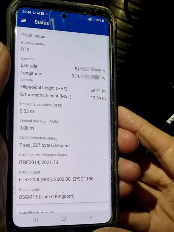
The lowest cost version of these better systems in 2021 is the Trimble Catalyst, which retails for around £360 plus delivery costs (this may be a little more for the DA2 model), and works as an external antenna attached to a phone. The location fixes can be down to 1-2 cm, with the NRTK subscription fees increasing along with the accuracy of the results. However, if readings are only occasionally needed, they can be paid for hourly at about £12 per hour (minimum 10 hours per year), which can work out much cheaper than an annual subscription, depending on how often it is needed. In personal testing, the accuracy is typically 2 cm horizontally and 3 cm vertically under a clear sky, while in a built up area with a lot of obstructions and reflections, the horizontal and vertical accuracy were both 3 cm. It took about 1 minute of initialisation to achieve that accuracy. The DA1 device uses GPS L1 and L2, GLONASS G1, Galileo E1, and QZSS L1 and L2, so it is dual frequency. The DA2 device can also use GPS L5, GLONASS L2, Galileo E5, BeiDou B1 and B2, and NavIC/IRNSS L5, as well as triple frequency SBAS. Being triple frequency for GPS means that the DA2 is better at eliminating atmospheric errors, but still gives the same performance with NRTK. Correctional data is updated every 2 seconds at the highest positioning accuracy, which is how it manages to get such good results in real time.
The Trimble Mobile Manager app settings allow you to switch the output between an ETRS89 frame that it calls "ETRF2000", WGS84 and ITRF2014 which all look useful for the British Isles, or one of several other national reference frames. In all cases, when using (N)RTK within Great Britain, the OS Net correctional data that Trimble VRS Now uses, is actually delivered in ETRF97 frame, epoch 2009.756 (that is a date, specified with a decimal point), but the Trimble Catalyst mistakenly thinks it is being delivered in ETRF2000 frame, epoch 2000.0. The Trimble Catalyst app therefore applies the wrong transformations when converting to other frames, giving a 5 cm error. As a result, when using NRTK with the Trimble Catalyst (which it will use whenever the phone has a data or WiFi connection), the output should always be left as "ETRF2000", so that the output coordinates are in the correct ETRS89 frame for British mapping. This bug has been acknowledged by Trimble, and a fix is being worked on. WGS84 is treated as synonymous with ITRF2014 current epoch (date). Selecting ITRF2014 for the output, however, will output coordinates in the 2010.0 epoch, so it gives the coordinates as they would have been in 2010, which is not useful for most purposes. The device can also use free or paid third party RTK sources, but it still requires a paid Trimble NRTK subscription to use a third party source, so it is not quite as accomodating as the Juniper Geode in that respect. Trimble refer to this as "positioning-as-a-service" or "receiver-as-a-service", meaning that you have to continue to pay to use the device's abilities, even if it is not Trimble that are providing the actual data. Renting the device's abilities, while pretending that you own the device.
Most of the higher priced devices come with their own software on board to record the data, and save it into a project. Android devices generally require you to supply your own software to record data. The accuracy is so high that it actually becomes difficult to find an app that doesn't truncate the output (most map apps think a GPS cannot give this level of accuracy, so they truncate the data at very low precision). There are very expensive apps designed for land surveying (such as ArcGIS), which are complex, and quite unnecessarily hard to use, since they expect you to be trained and doing this sort of thing every day. Far too many of them still insist on truncating the data precision, and many fail to save the altitude. However, you can use the GPSTest app from barbeauDev, and select the "Share" button, then enable "Include altitude" to see the full precision of the GNSS readings, and share them with other apps (or just take a screenshot!). Alternatively, the SW Maps app can record data at 1 mm precision; add a project, add a drawn feature layer for points, tap the pencil then "Record using GPS", and press the add button when ready. You can even enable averaging before saving a point, but it does not record the standard deviation or estimated error. Tap on points on the map to see their details. Export to other formats (such as GPX or KML) using the menu.
If you would like to set up your own base station, there are several options. Most of the major manufacturers make base station hardware, but this is once again likely to be very expensive. Typically, it is designed to work with their own devices, using radio frequency or the Internet to communicate with them. ArduSimple devices can also be set up as a base station (by adding a network connection module), which can be used either directly over the Internet or with a free caster service such as rtk2go to make the data available. This would then allow you and others to use your own RTK source, for free. Note that this is a bit technically involved. The standard installation instructions will always cause it to output WGS84 coordinates based on the day it was set up, which is perfectly fine when it does not need to be properly related to a map, such as farming. However, for mapping and surveying, it is not as helpful as ETRS89 in Great Britain, and means it needs to be reconfigured regularly to get it back in step with WGS84. It is therefore recommended that you use post processing with OS Net base station data, or a dedicated NRTK device, to initially determine your base station location in the correct reference frame for British mapping (ETRS89's ETRF97 2009.756). These coordinates can then be supplied as the fixed position for the device. If you allow the base station to compute its own position ("survey in") then you would need to convert the coordinates from WGS84 to the correct frame for British mapping. The software allows you to select a datum, but none match the reference frame actually used by British mapping.
Some lower cost GNSS units can use satellite-based augmentation (SBAS) to correct positions given by GNSS satellites, and the signal distortions that are caused by ionosphere fluctuations. (These systems are currently WAAS in North America, EGNOS in Europe and MSAS in Japan. India's GAGAN, Russia's SDCM and China's BDSBAS/SNAS are still in development or partially functional. South America's SACCSA, Africa's AFI, and Malaysia's unnamed system are still in the planning stage. There are also paid subscription services such as the global OmniSTAR.) Essentially this works in a similar way to NRTK, but with only a few base stations, and the details are relayed via satellites instead of via the Internet. This is only approximate, assuming that large parts of the country see the same errors, but it is better than nothing; within the British Isles, there are just 3 sites that check for distortion of satellite signals for the EGNOS system, with a total of just 40 sites across Europe. This correctional data can also be delivered by other means, such as radio signals; an example of this is Malaysia's SISPELSAT. However, this requires a second type of receiver for that signal, and the device must be able to access that second signal. Radio may work well in coastal areas, but can be blocked by mountains, and is absent in wide oceans. SBAS can work in most of the same places that GNSS can, without needing a second type of receiver. EGNOS data can also be delivered via a network connection for some uses, though proper differential GPS/GNSS will perform far better.
Note that some devices may claim to use satellite augmentation, but in actual fact may not see most of the augmentation satellites, or may never actually use the ones they can see. These will give the same results as a basic GNSS device without the feature. Often this is claimed to be because of obstructions or interference, since the satellites are geostationary, and sit relatively close to the horizon (33-24.5° above the horizon within Great Britain), positioned over the equator (EGNOS satellites are positioned over Africa). However, it seems to be down to the quality of the device, as better quality devices like the CT8 do not have that problem.
SBAS services may only provide augmentation for some of the GNSS constellations and not others. Typically, they do this if the GNSS constellation has more accuracy problems, such as the GPS constellation. This means that satellite augmentation may not be used if your GNSS device is set to use only a higher quality GNSS constellation (for example, EGNOS only augments the GPS constellation in 2021, and only the L1 frequency, but it is planned to have augmentation for Galileo in future too).
The Juniper Geode is an example of a device that makes the most out of SBAS. Without it, the device can achieve 1.2 metres accuracy, but its impressive 30 cm accuracy relies on SBAS. The Trimble Catalyst also uses SBAS when its NRTK and RTPPP correction sources are not available, and the accuracy in such conditions is stated as 50 cm. With the Catalyst, a paid subscription is needed in order to use SBAS (even though SBAS is a free satellite service that other devices use without any subscription, so once again you would be paying to use free data). ArduSimple devices can also use SBAS to obtain an accuracy of around 55 cm horizontally and 70 cm vertically (CEP), which they mistakenly label as "DGNSS" when describing how the fix was made.
Dual or multiple frequency devices can also use the two or three frequencies emitted by most GNSS satellites to work out how much the signal is being diffracted by the ionosphere, and work out the correct timing of the signal. In some devices, this can give similar accuracy to satellite augmentation, and can help detect more localised ionospheric distortion, if the satellites offer multiple frequencies. Devices may also use it to help detect reflections from buildings or landscape ("multipath"), and discard reflected signals. However, it does not detect other things like satellite clock or positioning errors, which standard augmentation can help counteract somewhat. As a result, both satellite augmentation and dual frequency still serve a purpose.
Currently all GNSS constellations have at least 2 "L-band" frequencies, and most of them share the L1 and L5 frequencies used by GPS (though each constellation may give them different names), with some having other frequencies in between. GLONASS is the exception as its frequencies are different from all other constellations. Most consumer grade dual frequency devices use L1 and L5, while professional grade devices might use L1 and L2. GPS L2 was previously for military use only, and did not carry a standard signal, but industrial grade devices could use the data pulses to work out ionospheric distortion even if they could not understand the message it contained. As of 2021, less than half of the GPS satellites emit the L5 frequency (but all emit L1 and L2). As a result, more than half of the GPS satellites appear to be single frequency to most consumer grade devices; SBAS can correct those, but L1+L5 dual frequency cannot. Almost no consumer grade devices can use the second or third GLONASS frequencies, so they treat it as single frequency. NavIC/IRNSS only offers the L5 frequency within the normal range that consumer grade devices can use, though the L1 frequency is also due to be available soon. NavIC/IRNSS does currently have a second frequency in the S-band, the same range used by Wi-Fi and bluetooth (so it can suffer from interference near devices that use those frequencies). Most consumer grade antennae are not configued to receive S-band signals.
Note that some manufacturers may use the terms dual-band or multi-band for this feature, which confuses it with multi-GNSS. Some, such as Garmin, have used the same term for these two unrelated features in different devices in their range, so when selecting a device, check what it really supports. Technically, both features can rely on a device supporting more than one frequency, as the two most commonly supported GNSS constellations (GPS and GLONASS) use their own frequencies, which is where the confusion arrises.
As of 2020, the Juniper Cedar CT8 has one of the most complete implementations of satellite augmentation (within Europe this will use EGNOS, so it only augments the GPS L1 frequency), dual frequency correction and dual constellation, and generally gives readings with far better accuracy than a typical GPS/GNSS unit - within 1 metre CEP (approximately ±1.2011 metres standard deviation) in many tests. It retails for a little over £900 by the time you add tax and shipping. It also copes fairly well around buildings and under trees, detecting and rejecting reflected signals better than many other devices. Users can choose which two constellations to use in the location settings. GPS and Galileo gives the best dual frequency support; GLONASS is not bad, but since it is not dual frequency, it randomly gives results with higher errors, especially for altitude, while Galileo has the best accuracy of all public systems. Note that when using GPS+Galileo mode, all apps show Galileo satellites as if they were GPS satellites - this is a quirk seen only on the CT8 tablet, the same apps show those satellites correctly on other devices. In spite of it being one of the most accurate available, the vertical accuracy can sometimes be disappointing as it fluctuates constantly. Often the results of averaging are within 1 metre, but during testing, 5 hours of averaging once saw a 3 metre vertical error in the final position.
Military GNSS devices are sometimes suggested as being better, but this is mainly because they are dual frequency, while most civilian ones are not; it first became available for civilian use in 2005, but only became available in basic GNSS devices like some phones starting in 2018. Military devices may also use encrypted channels, but this is used to prevent fake signals from being able to confuse them (signals can still be jammed), rather than to improve the accuracy. A dual frequency GNSS device which uses satellite augmentation can provide good results, even if it is not a military device.
Note that although the Samsung Galaxy S20 and S21 series typically have dual frequency GNSS support in the "Plus" and "Ultra" models, they must not be used for locating surveys, for reasons mentioned in the section on GPS/GNSS averaging. This is unfortunate, as they are some of the first commonly available consumer grade phones to support dual frequency. They can still be used for post-processing, however.
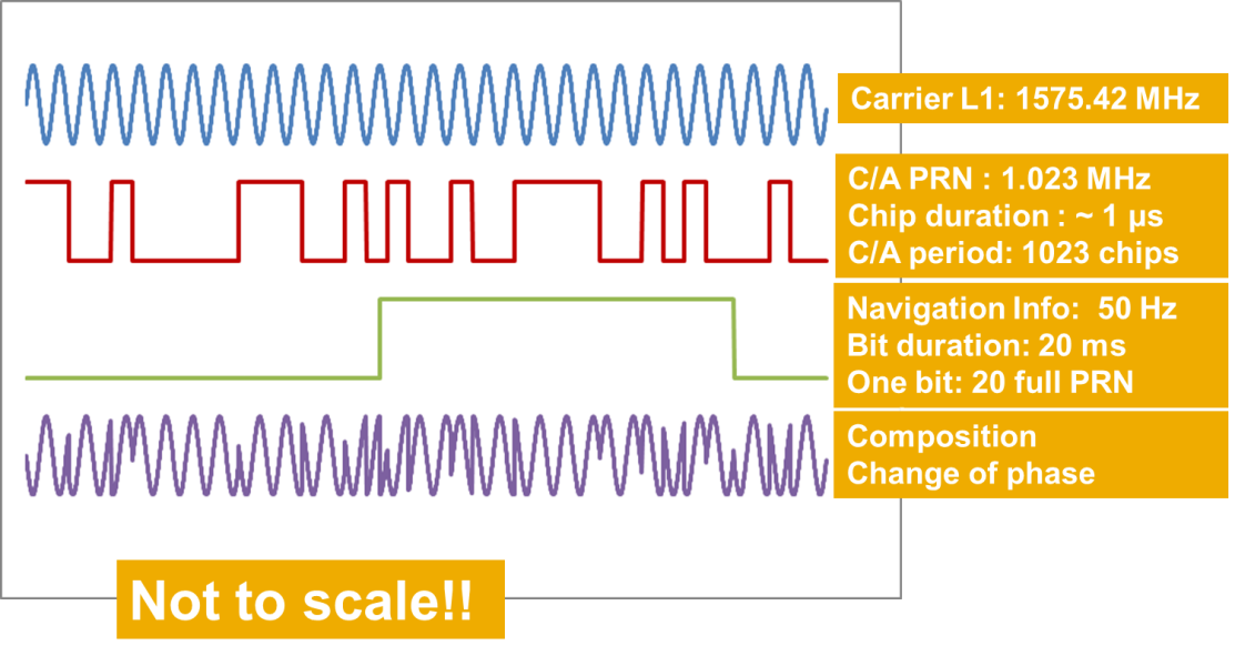
GNSS signals are binary data sent using phase modulation of a carrier frequency (don't worry if you don't understand this part, it's not important for locating a cave, it's just interesting from a physics perspective), and GNSS devices try their best to align the binary messages sent by the satellites with their own generated messages. The timing differences are used in the position calculations, and little mistakes in alignment can cause significant errors in the calculated positions.
With carrier phase tracking, a GNSS device then tries to align the waves of the carrier signal itself as well, improving the alignment of the main signal in the process. If they can work out exactly how to align the carrier frequencies, the accuracy can be improved to within a few centimetres. This is quite difficult to do, because the carrier frequency does not have any obvious shapes to align - it is a normal sine wave, since it was not intended for this purpose, and distortions can make it look strange. However devices can still try to align it, with varying degrees of perfection; the better they are, the more they are likely to cost.
This technique is combined with satellite augmentation by the Juniper Geode and higher quality systems like the Leica Geosystems GS14 to provide better accuracy, even when not using NRTK. The Geode relies mostly on this approach and satellite augmentation to get its accuracy, without being dual frequency, which gives an idea of how effective this can be. When using just carrier phase tracking, the Geode can achieve 1.2 metres accuracy from a single frequency, which is a lot better than most basic dual frequency devices can manage.
It is possible to determine position using a single satellite, by very carefully monitoring its frequency. While it moves towards a receiver, the frequency observed from the receiver will be slightly higher. While it moves away from a receiver, the frequency observed will be slightly lower. As it passes your latitude, the frequency shifts most dramatically. As the Earth rotates you past its longitude, the frequency also shifts, with the effect most pronounced at the equator. Even if it is not passing directly overhead at the current moment, a few minutes of observations can be enough to detect both frequency shifting effects taking place. Knowing how fast the satellite is moving in its orbit, and how fast the receiver was moving towards it or away from it due to the rotation of the Earth and the orbit of the satellite, some very complicated mathematics can reveal a position, accurate to around 100 metres.
This only works well for stationary or slow moving receivers, so is not particularly useful for standard GNSS usage. However, it was enough to be used by the very first satellite navigation systems of NNSS/Transit and Tsiklon. (At the time, 15 minutes of subsequent computations were needed to calculate the position from the data that had been gathered.) It works best for satellites in polar orbit (which none of the major GNSS satellites use, but the original systems were). Nevertheless, this data is still recorded by many systems for use in post processing, which can help with motion prediction of the GNSS device.
Satellites are not perfect. They are supposed to follow a predictable orbit around the world, always in perfect circles or ellipses. But sometimes they get out of that perfect orbit and have to make small adjustments with their thrusters to try to get perfectly back in line - corrections will be needed repeatedly because perfection is impossible. They might have to step up or down around pieces of space junk, such as the remains of damaged or non-functioning satellites. The orbits also relate to the centre of mass of the satellite, not the position of the satellite's antenna (or the point in the antenna where the signal appears to emanate from - its phase centre). The antenna is usually slightly closer to the earth, but the exact amount will depend on the satellite's orientation.
The satellites have very precise clocks that they rely on for computing the timing of the messages that they send out, but due to their speed, the effects of gravity, and changing orbits or speeds during manoeuvres, the clocks can get affected by the time shifts caused by general and special relativity. When something moves faster, it experiences time more slowly, and the Earth's gravity causes spacetime to be significantly curved, so time slows down more at the Earth's surface than it does at a satellite's orbit. GNSS satellites experience differences in time compared with Earth, because of their speed (-7µs per day) and the effects of gravity (+45µs per day), compared with the speed and gravity of the Earth's surface. Overall, a GNSS satellite sees time move faster by around 38µs per day when it is not manoeuvring, equating to about 10 km of positioning error if it were ignored, so the satellite adjusts its clock to take account of that difference. However, the adjustment needs to change whenever it manoeuvres, and due to modelling limitations, there are imperfections in the adjustments.
In addition, the satellite's hardware or software might respond unexpectedly slowly when it is processing instructions for sending messages. These orbit errors, clock errors, and other timing errors can cause a code bias or phase bias (depending on whether they affect the standard code message or the carrier phase), and can cause little delays or early arrival of the signal sent out by the satellite, which make a GNSS device think it is further from or closer to the satellite than it really is. The effects of these tiny errors is more pronounced at equatorial latitudes, where the speed of the Earth's rotation is highest.
These little mistakes can be measured from base stations around the world, and the corrections can be sent in realtime to a GNSS device, known as state space representation (SSR). (And yes, that means that they literally point lasers at the satellites to measure their positions.) The device can then apply the corrections to the satellite signals it is seeing, and use that to refine its calculated position. This is known as real-time precise point positioning (RTPPP). It results in a substantial improvement to the position, potentially down to 3 cm accuracy or better, depending on how well the errors can be calculated, how quickly they can be delivered after that calculation, how often correction samples are delivered, how many corrections can be processed by the device, and whether the carrier phase is also corrected. In practice, this may not be quite as accurate as NRTK (Leica show an accuracy of around 3 cm horizontally and 6 cm vertically in their documentation), though with some devices, the difference can be minimal. The main remaining source of error is that the ionospheric and tropospheric distortions are not compensated for, so the device needs to calculate this itself using dual or triple frequency. Reflections/multipath also cannot be compensated for, unless the device can detect and counteract it with dual frequency. The device itself can also have its own processing latency or other biases, which cannot be compensated for, but that can happen with RTK and basic GNSS devices too. Unlike RTK, the data is not specific to the device's location, so it is possible to send it via satellites or network connections. Leica/HxGN/Hexagon SmartLink, Leica/HxGN/Hexagon/NovAtel TerraStar, NovAtel CORRECT (PPP mode), Carlson Atlas, Trimble RTX and Topcon Topnet L-Band are examples of providers who offer this sort of service, but the fees are very similar to the subscription fees for RTK - often it comes as part of the same subscription, so the device can use NRTK or satellite-based RTPPP depending on whether a network connection is available. Trimble RTX, NovAtel CORRECT, and some of the TerraStar service levels are actually a slightly enhanced version of RTPPP, as they also contain a global ionospheric model made without using base stations (this model is not based on instantaneous measurements, but it works well enough to speed up initialisation).
The Trimble Catalyst is again the lowest cost option here, as it can receive this data via Trimble RTX over the Internet in areas where NRTK is not available, and via Trimble RTX satellites whenever there is no network connection. This service is available at no additional cost via any of the subscription levels. When using RTPPP with the Trimble Catalyst, the correctional data is actually delivered in ITRF2014 (current epoch), and the position is then transformed into the other reference frames on demand. WGS84 is again treated as synonymous with ITRF2014 current epoch. It is worth noting that when it outputs coordinates in ETRF2000, it uses that actual frame in epoch 2000.0, not the ETRF97 frame and epoch 2009.756 used by OS Net to represent ETRS89 in Great Britain. This can introduce a roughly 5 cm error when converting it to a grid reference. Therefore when using Trimble RTX with the Trimble Catalyst, it is actually better to output the coordinates with the WGS84 option selected, and use the HowToCreate High Accuracy conversion tool to convert it to ETRS89. This limitation has been acknowledged by Trimble, and a fix is being worked on; hopefully, it will be possible to select ETRF97 2009.756 in future.
It is worth checking the coverage areas for each service provider, as each will have limitations (largely because they normally use geostationary satellites). For example, as of 2021, Trimble RTX does not cover the northern parts of Scotland, Scandinavia, Iceland, Greenland, Canada, Alaska or Russia, or any of Antarctica. This also means that when relying on this service via satellites, the device needs to have a clear view of the sky towards the equator. Just like augmentation satellites, these typically sit 33-24.5° above the horizon within Great Britain.
RTPPP generally takes a little longer to establish a stable position. A high quality device might need several minutes to monitor the effects of ionopheric/tropospheric distortion before it can give a stable output. Depending on the device, the output may continue to improve over time, as it refines its position better. Leica's documentation suggests that their devices can switch from NRTK to RTPPP without any delay if they have spent at least 3 minutes observing the SmartLink satellites first while using NRTK. It takes the same devices about 10-30 minutes to refine their position to the same accuracy when starting from scratch with only RTPPP. After losing the satellite signal, it takes about 1 minute to regain accuracy once the satellites become visible again. In personal testing, the Trimble Catalyst took between 2 and 5 minutes to get an accuracy of 3 cm horizontally and 8 cm vertically, which is close to its stated best accuracy of 2 cm horiontally and 5 cm vertically. However, this was tested in an area where Trimble RTX Fast is available (more details below), so it is epected to be much faster than basic RTPPP. The updates seem to be sent every 5-10 seconds via the Trimble RTX system, using around 2.2 kbps (though the maximum data rate can be about 14 kbps). Carlson state a 2 cm maximum accuracy, with 10-40 minutes required to reach that accuracy level.
There is also the possibility to combine the approach of RTPPP with some of the base station reference data of NRTK. In this case, the base station data only needs to specifically correct ionospheric and tropospheric distortion, which were missing with RTPPP, largely removing the need for dual frequency. This is called PPP-RTK. It has the advantage that it does not need a base station to be as close to you as standard NRTK does, because it can model the likely ionospheric distortion in between; 200-300 km is easily possible. Trimble use an average spacing of 200 km within Europe, with just 23 stations needed in Great Britain, a fifth of the number needed for NRTK. A device that uses PPP-RTK can initialise far faster than a device that uses basic PPP, usually around a minute to full accuracy. It can use lower bandwidth, but still relies on a network connection or dedicated satellite broadcast covering a specific area, since the data does have to be specific to your area, even if it is less specific than NRTK. In general, a satellite service can cover an entire continent (high latitudes are difficult), given the smaller amount of data it needs to send.
Trimble RTX Fast is a PPP-RTK service available in Europe and the USA, which the Trimble Catalyst will use when using Trimble RTX via an Internet connection from those areas. Trimble RTX Fast supposedly takes about 1 minute to reach full accuracy, but in personal testing took between 2 and 5 minutes with a Trimble Catalyst. Sapcorda/u-blox is an example of a PPP-RTK provider, using the SPARTN format over their PointPerfect/SAPA service, supplied via a network connection or L-band satellites. Accuracy is about 3-6 cm horizontally, and the service covers Europe and the USA. It requires a subscription, with several pricing options depending on how often you want to use it (under £3 for 60 hours per month), and the L-band satellite version is just £22 per month, assuming you can find a device that can use it. The ArduSimple devices can use PPP-RTK, but an additional board is needed (with an additional expense). ArduSimple's simpleSSR costs £340 per year, using PointPerfect data. SimpleSSR has the limitation that it requires a network connection, rather than using satellites, which unfortunately removes one of the major advantages of PPP. ArduSimple devices do not currently support satellite based PPP-RTK (as of 2021).
Galileo High Accuracy Service (HAS) is due to become partly available in 2022 and fully available in 2024, which will offer RTPPP for free around the world, both via satellite and network connections. And there will be much rejoicing. Even a low cost device will then be able to perform RTPPP, giving around 20 cm horizontal accuracy, and 40 cm vertical accuracy. The free global service should take around 5 minutes of readings to obtain that accuracy. The service will only correct the GPS and Galileo constellations, but that is all that will be needed to perform RTPPP (other constellations can be ignored). Within Europe, it will use PPP-RTK, which allows it to take less less than 2 minutes to reach full accuracy. An equivalent service is already avaiable in Japan.

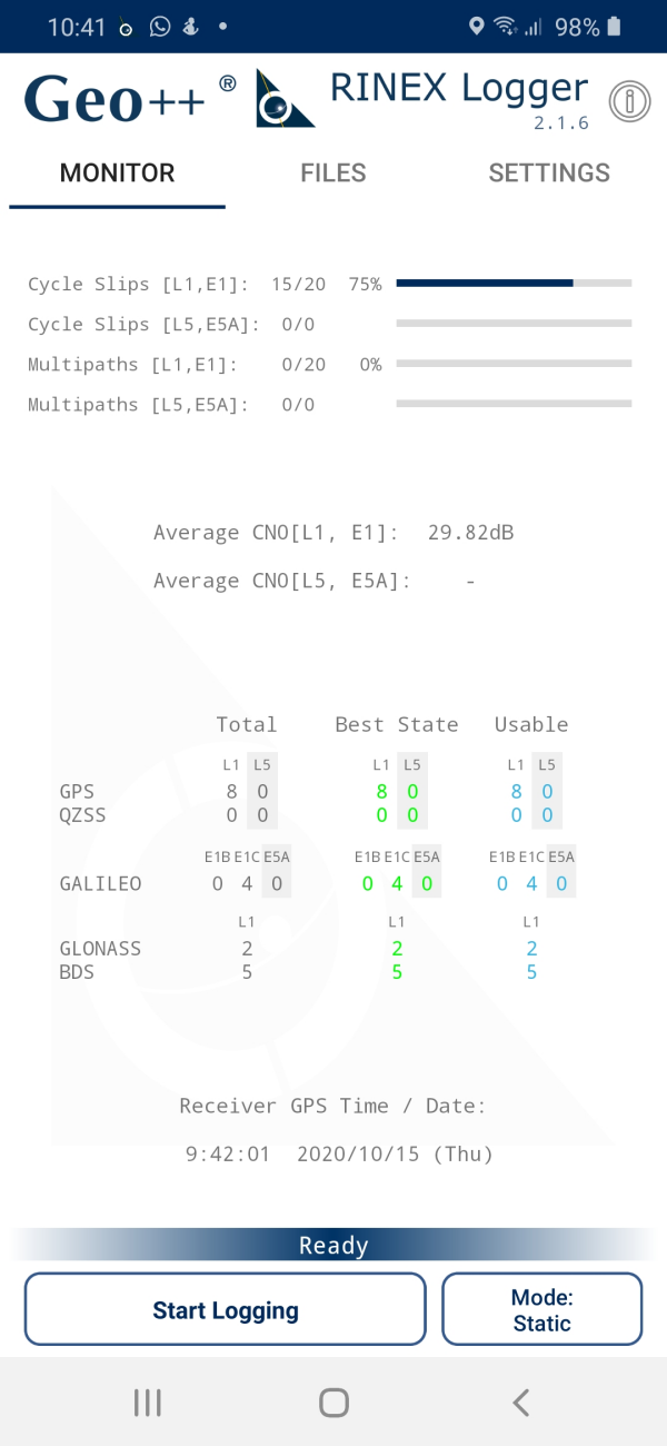
Some devices can collect the raw satellite data in RINEX format, which can then be post-processed on a computer in several different ways. It can be processed in the same way as GPS/GNSS averaging, using almanac (expected satellite position) data which is made available in advance every day, and ephemeris (detailed satellite position) broadcast by the satellites. However, this usually gives results that are no better than simply performing averaging on the device, and therefore is not really worth the effort. Kalman filtering can improve the results slightly, just like it can when performed on the device.
To improve results, the data can be processed to perform carrier phase tracking even if the device itself could not do it natively. A post-processing application can use precise satellite clock, orbit and bias error data that is made available 12-24 hours after the readings were taken, from measurements taken in observation stations all around the world. These approaches are known as Precise Point Positioning (PPP). For best results, the GNSS data needs to be collected for several hours (5 is a good number) from a static location, the device should be dual frequency, and it should support multiple constellations - the more data it can gather, the better. Depending on which approach is used, and how good an application is at it, it can be extremely effective, down to a few centimetres. Many services charge a fee for PPP, but there are a few free ones. The majority of applications that can do PPP are incredibly complicated, and usually require you to download a lot of files from public data sources, for which you need to know exactly which files you need. Some can locate the files automatically for you. The applications may take a lot of effort to configure and use correctly, so training is usually required. However, there are a few simpler services that can do it for free, automatically downloading the appropriate files, and processing them.
RINEX can also be post processed using augmentation data from a base station, which is also delivered in RINEX format - this is known as Post-Processed Kinematic, or PPK. This is much less convenient than a system that can give accurate results in realtime, but is sometimes used by RTK systems that are being used in an area without any network connection, and therefore do not have access to their RTK data source. It may also be used when initially setting up a local base station so that you can use it for your own rovers. RINEX data is provided for free by Ordnance Survey and EPOS. RINEX data subscriptions for other services can cost around £450 per year.
With PPK, the GNSS devices that gather data may in theory be of lower cost and quality than industrial NRTK devices, effectively turning a low cost device into a post-processed differential GNSS. RINEX export is available on some dedicated handheld GNSS devices and the newest Android phones that we tested, but not on a CT8. The accuracy will depend on the quality of the data logged by the GNSS chip, but in theory, positions may be calculated to within as little as 10 cm from a handheld device. Phones present some challenges, because of the power saving tactics that they might use. Lower quality devices generally pick up a lot of reflected signals, or fail to collect the full amount of data available to them, which leaves the post processing application with a lot more work to do. A high quality antenna can improve matters. In an ideal situation, the base station should offer sampling rates as high as the device, typically one sample per second, but post processing can work with base station data that updates every 30 seconds or so. A few hours of readings will be needed to get the accuracy to within desired levels when using a low quality device, or when using base stations with a low sampling rate; 2-5 hours is a good start. Longer times might be needed for longer distances from a base station, and longer times might be needed in equatorial latitudes to allow for the exaggerated effects of satellite clock/code biases and ionospheric fluctuations.
If data is not gathered for long enough (such as 10 minutes), or if the device randomly ignores data in order to save power, the error will be as bad as regular GPS/GNSS averaging with the same device. This shows that post processing with a poor quality device is not a real replacement for a high quality differential GNSS, since a high quality device with NRTK normally needs only a couple of minutes to get excellent results. The device needs to be able to log RINEX data without any interruptions, something which is surprisingly difficult to do with a phone. Unlike with PPP, the device does not need to be dual frequency, since the base station can help detect ionospheric distortion of the signal. However, the results may be a little better if the device and base station both support the same dual frequencies, particularly at times or places where ionospheric distortion is most severe. When testing using either single or dual frequency in the British Isles, with base station data that had a sampling rate of 30 seconds, results of a 2 hour data collection from a low quality handheld device were accurate to within under 10 cm. When testing in Indonnesia, base stations under 20 km away were not able to counteract the more severe equatorial ionospheric distortion, and the accuracy achieved with single frequency data was around five times worse than in the British Isles. It should be noted that either of these results are substantially better than anything that can be achieved by standard GPS/GNSS averaging in the same locations.
Neither PPP nor PPK can eliminate the limitations of a low quality antenna, or poor placement of it. In areas with large amounts of reflected or blocked signals, such as near buildings or cliffs, or under trees, much longer data collection might be needed, and the results may still have a substantial bias. Getting below 1 metre accuracy might not be possible when using a low quality device. The best results obtained during personal testing were on top of a mountain with a clear view. In a British suburban garden surrounded by houses, 5 hours of sampling managed to get the horizontal accuracy down to within a metre, but the vertical error was several metres.
Many features rely on the device and base station collecting data in RINEX 3 format. Some older devices can only export data in outdated versions of RINEX 2. Most devices that export RINEX 2 do not support carrier phase tracking, Galileo, BeiDou, QZSS, IRNSS/NavIC, GPS L5, SBAS, or several other types of recorded data. Some of it can be exported in RINEX 2.11, but a device that supports RINEX 3 can give much more detailed information. Carrier phase information can be exported in fairly low detail by devices that support RINEX 3, and while that cannot be directly used to improve readings, statistical analysis can be used by some software to correct the carrier phase alignment and improve the readings dramatically. When looking for a device to use, aim for one that exports RINEX 3. You might not have any control over the base station data, however.
For instructions on how to do post processing, see the section on post processing a RINEX file below.
This section covers features that can cause poor results or misleading results.
With A-GPS, a mobile phone service provider can send a subset of the GNSS signal data over the mobile data connection, rather than the device having to collect the data directly from the satellites. In this case, the phone network knows roughly where you are already because of which cell towers you are connected to, and can select the right satellites for you. Your phone does not have to wait for the GNSS satellites to send their orbit data (almanac and ephemeris) in order to locate them and their frequencies. Instead, the phone network can send you the satellite location, orbit, and approximate time information immediately, which it has been monitoring constantly, and your device can use that data to get an approximate location fix, work out expected information about the satellite such as its frequencies, and speed up subsequent fixes which are taken directly from the satellite. As well as being faster to get an initial location fix, this is also useful in places like buildings, where the phone data signal works well, but the satellite signals are blocked.
A-GPS is not, however, designed to improve accuracy. In fact, it does the opposite, reducing the accuracy during the time it is being used. Your GNSS device will not actively tell you whether the location data comes from A-GPS or real GNSS, and you will not know whether the location data you are currently receiving is trustworthy enough to use. You should therefore make sure that if your device has A-GPS support, that it is disabled when you are trying to get location fixes for surveying. You need accuracy, not speed. Some Android devices offer a location setting to allow you to choose between using only the device sensors, or using other methods as well. Some Android devices do not have a way to disable it, and instead, you need to disable mobile data.
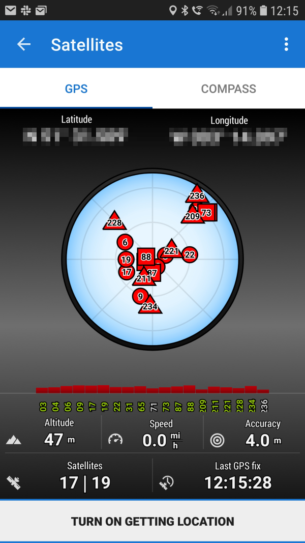
Some devices may supplement their altitude data with barometric data, or may use that method exclusively. This is because over short time spans, barometric pressure does not jump around as much as the altitude seen by a lower quality GNSS device (especially one that is moving), and when recording a track, it gives a more realistic altitude profile. The idea is that you calibrate the altitude beforehand at a known point such as a benchmark, quickly get to the desired location before the local air pressure changes due to weather effects, and then the device calculates the likely height from the difference in air pressure caused by altitude. When testing this on a day with fairly steady pressure, against an ascent of 190 metres from the benchmark where it was freshly calibrated, the device had miscalculated the altitude by 23.5 metres; an error of over 12%. This sort of error is unacceptable from a surveying perspective, and devices that use barometric altimeters should therefore be avoided.
Aircraft and some devices can use ground-based pressure monitoring stations to correct their altimeter's pressure calibration along their path, but these cannot compensate for the effects of inclement weather and temperature inversions, uplift over mountains, temperature fluctuations as the device moves between sunlit and shaded areas, or local pressure disturbances. These disturbances can amount to several hundred metres of error, and results therefore cannot be trusted for surveying. These altimeters are designed to be used in normalised pressure and temperature gradients experienced at high altitudes, when elevated significantly off the ground.
Devices may choose to display GPS altitudes (which is generally what is needed for surveying with a GPS), or may augment it using a geoid model or Helmert transformation, sometimes stated as MSL or Mean Sea Level. A geoid approximately represents the fluctuations in gravity around the world. Think of it as the level that the ocean would be at if the land was all removed, and there were no tides or winds, so it can be subtracted from a GPS altitude to give an approximation of the height above sea level. There are many models available, but the most common one is EGM96. The resolution is relatively poor; one sample point every 28 km (by comparison, Ordnance Survey apply one correction for every 1 km grid square), and even the high resolution version still only gives one correction every 9 km. A geoid model does not take local tidal effects into account, so it does not accurately represent the height above the tidal datum used by a mapping agency; tides are effected by narrow sea channels and ocean currents, which is especially important around the British Isles. Alternatively, devices may approximately convert altitudes to a local mapping datum using Helmert transformations. In Britain, this can introduce as much as a 3 metre error when using the common Airy1830 ellipsoid as a reference. Any such augmentation needs to be removed in order to get back to the actual GPS altitude. These augmentations do not improve accuracy, they make the results far less accurate instead.
Other devices may ignore GPS altitude entirely, and rely instead on a terrain map with approximate altitudes, known as a digital elevation model or DEM. Typically, this will be used by GNSS trackers, such as watches that do not include a barometer, but some apps on Android, such as ViewRanger, also use the same approach. The terrain map is similar to what is used by 3D maps like Google Earth, and is typically generated from LIDAR scans (SRTM), with a geoid height subtracted from it. As a result, the values it gives are no better than if you picked the altitude from the maps directly. Often, the position will be taken from the top of any trees above you, or more likely somewhere in the surrounding area, depending on the LIDAR resolution and accuracy. Devices that use this approach typically do so because of how poor their GNSS receivers are, and therefore should not be trusted for their horizontal positions either.
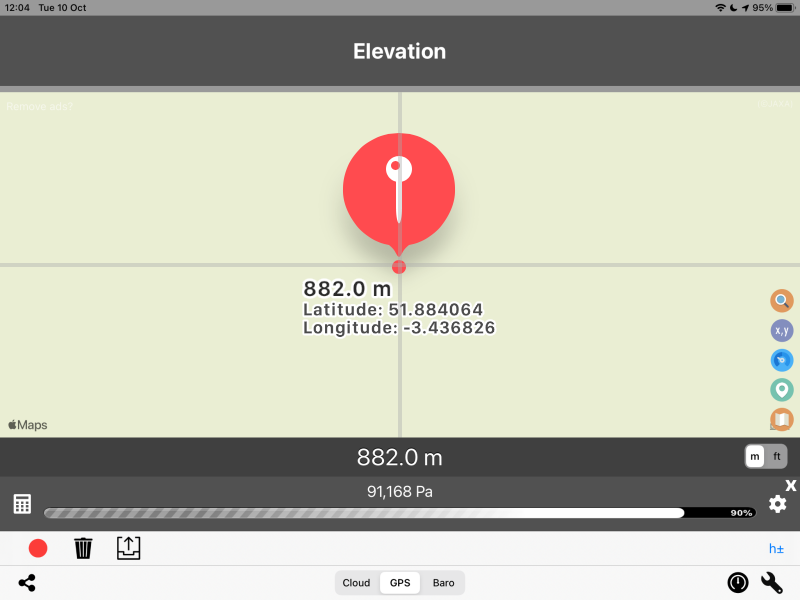
iOS devices such as iPhones and iPads use a terrain map when claiming that they are using the GPS, or a barometric altitude if the app asks for it (which needs to be regularly calibrated manually - it tries to compensate for temperature, but fails rather badly in practice). There is no way to disable this in the settings, and any apps that try to show GPS (ellipsoidal) altitudes will be making a guess as to which digital elevation model might be in use (it appears to be the 1 arc-second - approximately 30 metre resolution - global data set with interpolation in between), and then which geoid height they might need to add to the terrain map in order to show a GPS altitude. As a result, all iOS devices are absolutely unusable for surveying. However, external antennae might have their own way of presenting height data to the device, and it might actually be possible to use those. You will need to check the information for the specific antenna and apps designed for those antennae.
Mobile devices may also use local Wi-Fi and Bluetooth data to get a location fix. Geolocation service providers either use data collection vehicles or other people's mobile devices to gather details of the Wi-Fi network names and hardware identifiers, and Bluetooth device identifiers that are broadcasting in each neighbourhood, and how strong the signals are. When your device wants to get a location fix, it can gather details of these networks and devices that it can detect, and send them to a location service provider. It can record signal strengths, or even the time it takes to send and receive data from those devices (Wi-Fi RTT), to further refine the distance from them. The location service provider responds with an approximate location where it believes you might be able to see those networks and devices, with those signal strengths. Apart from being a massive privacy invasion (this approach is banned in some countries), the location returned is hopelessly approximate, often 100 metres or more wrong in densely populated areas, and completely absent in the countryside. Wi-Fi and Bluetooth infrastructure is generally distributed horizontally (except in tower blocks), so the positions that can be calculated by these methods are practically useless for establishing altitudes. In spite of its limitations, this is the approach that is normally used by Web browsers for geolocation on devices without GNSS support, and many mobile devices also use it alongside their GNSS sensors. In places with fixed architecture and services, such as shopping centres, this can be much more accurate, depending on how well the infrastructure has been mapped out by the location service provider, and how often the infrastructure gets moved or changed by the owners of the building, but that does not help at all in the countryside.
In cases where a location provider cannot find anything useful in the data your device gathered, it can use your device's IP address to approximate the position, based on where your network provider has registered that IP address, or an IP location database has guessed that it might be, based on the hostname or other details provided by your network provider. This often gets a location in the right district of a city, but sometimes can be positioned in the wrong country, if an IP address block was recently sold to another company. It is usually complete nonsense in countryside areas.
Alternatively, a mobile service provider may send your device an approximate location estimation, based on which cell towers can see it. This is a rough estimate within about a 3 km radius, and can be affected by obstructions and cliffs.
Devices or external service providers can use other techniques to identify location, such as communicating with local Bluetooth devices that broadcast local positioning information. They may also use motion prediction from previously known movement, or from inertial measurements. In extreme cases, they may use other sensors such as camera lighting, identifying objects or landmarks in camera images, recognising types of echos detected by the microphone, or analysing a magnetic compass in the device, to decide if you are moving, or if your location matches a known location. These approaches are known collectively as an Indoor Positioning System. While this may be useful in a building (or creepy - they are used for surveillance), it does not serve the desired purpose of locating a cave survey, and could give unpredictable results as it tries to make sense of the conditions below a cliff or tree canopy.
Needless to say; if your device can use any of these features for determining its location, you should disable those options in its location settings. You want an actual location, not an approximate guess made by any of those methods. If you suspect that your device uses any of these approaches, and you cannot find any ways to disable this on your device, then do not use that device for locating cave surveys. On Android, you might find some options in the location settings. The Juniper Cedar CT8 is an example of a device where the location settings allow you to tell the device to obtain location data only from the GNSS sensor, not from the cellular network, Wi-Fi or Bluetooth.
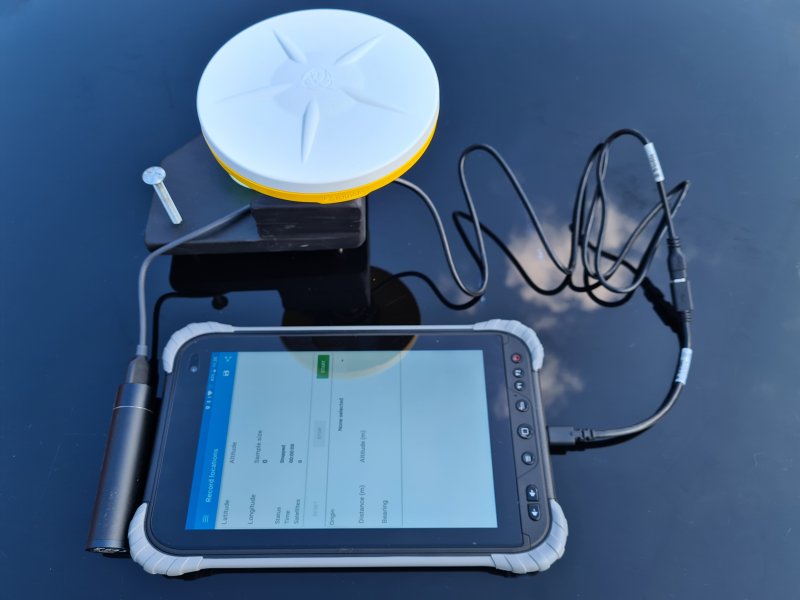
There are a few factors to consider; how accurate you need the location fixes to be, how often you will need to obtain location fixes, how much time you are willing to wait for each location fix, how much money you are willing to spend, and whether you will have a network connection available. The best systems will be those that can use RTK, NRTK, RTPPP or PPP-RTK, and many cave surveyors would be very happy to own such a device. They will also normally be the most expensive, but there are some impressively low cost options available. Post processing can also get similar results from a low quality device, as long as enough time is available to take readings. Averaging also takes time, but gets comparatively worse results. A better device or antenna can produce better results when averaging.
A system that uses RTK often does not need to have all of the other features in order to give an accuracy within a few centimetres, but in places with no access to the Internet for RTK, the other features become very useful for getting an accurate reading. Usually, this takes some time for the device to monitor the satellite responses in its area, and build up its own correction data which it applies to readings taken from a handheld controller - the main unit then becomes your base station. This approach is used in many devices aimed at industrial usage, such as those made by Leica Geosystems, Carlson, Trimble and Topcon. The best systems would combine all of the features at once, such as multiple GNSS constellations, dual frequency, satellite augmentation, carrier phase tracking, NRTK and RTPPP or PPP-RTK, with a high quality source. For example, the Leica Geosystems GS14 is one such system.
These NRTK/RTPPP devices can sometimes be bought second-hand from a rental supplier, but the RTK/RTPPP subscriptions would still be needed. If you will need it to work in a place without any phone signal, then a device that can use satellite-based RTPPP or PPP-RTK would be needed, or post processing with RTK data could be performed afterwards. If you want to get the most accurate location fixes for a survey, and you don't have the time to do lengthy GPS/GNSS averaging or RINEX capturing, you may want to rent or buy one of these systems. Rental of a differential GNSS is usually £300-500 for a weekend in 2020, and you will normally need extra time to learn how to use it properly. Sadly, these are out of the price range for most cave survey projects, and even their rental costs may also be considered too high. The Trimble Catalyst is, however, relatively low cost, and its subscription costs can be very low if it is only used infrequently. Its purchase cost is about as much as a single rental cost of a typical NRTK device.
Products without RTK, RTPPP or PPP-RTK but with several other accuracy improving features can often serve the purpose for cave surveys, using GPS/GNSS averaging to get a better estimate if that is needed. If they are too costly, you may have to do GPS/GNSS averaging for a lot longer with a poorer device, and still have fairly inaccurate results. It is worth noting that when using a Trimble Catalyst - one of the highest grade devices available within a hobbyist's budget - without any correctional data, it still showed the position wandering around in a 3.25 by 2 metre radius ellipse, over a 10 metres vertical range, all while stating a 2 metre RMS (2.1 metres vertically) accuracy. (When used without a subscription, the Catalyst's stated accuracy is artificially limited to a minimum of 2 metres; the device could in fact be estimating a better RMS accuracy.) 3 hours of averaging still gave an error of about 1 metre horizontally and 3 metres vertically. A Juniper Cedar CT8 had a 5.5 by 4 metre radius ellipse, and 18 metre vertical range, while claiming 1 metre horizontal and 1.9 metres vertical accuracy. Filtered averaging or post-processing is needed even with high quality devices when NRTK, RTPPP and PPP-RTK are not available.
While a basic phone is not a recommended device for averaging, one with enough GNSS accuracy improving features might be considered good enough if it proves to be accurate during lengthy testing, and does not apply motion smoothing or filtering of its own. As of 2020 though, none are quite as capable as a Juniper Cedar CT8, or a Juniper Geode. If you are looking to purchase a good device that does not need a costly subscription, these would be my recommendations.
It is perhaps surprising that some of the dedicated handheld GNSS devices shown in this article fare relatively poorly in spite of having features like multi-band, satellite augmentation or dual frequency, and GPS/GNSS averaging. Largely this is down to them rounding values or truncating precision (which cripples their results when averaging), but even so, the stated accuracies were overestimated, and the actual results were quite poor to an amount that could not be explained by rounding or truncating. Given all of the problems mentioned in this article, a handheld device whose position has settled so that it claims "1.8m" on the screen, could actually be giving a position with a horizontal error of over 20 metres, and perfect averaging (which is an impossibility) might only be able to bring that down to 13 metres, or 8 metres with high accuracy conversion routines (the actual errors depend on where you are in the country - these numbers are for the worst case in the British Isles, the errors can be larger elsewhere). That is ignoring the bias caused by reflections. In fact, some phones without those features seem to get better results, closer to known positions. The altitude measurements given by these devices are shockingly bad (quite frankly, any device whose altitude uncertainty is 244 metres, is not a tool that should be considered for surveying). This article mentions the popular Garmin devices because these are what many outdor enthusiasts in the UK use (and cavers often take them on expeditions), but many of the problems can be seen on other brands too, where similar design choices have been made in the software on the device. These handheld devices are intended for recording long tracks like walking or cycling routes, and navigating to a destination in harsh conditions. They were never intended for use in surveying, and they are not well suited to that purpose.
If you are able to learn how to use post-processing, the best devices will be the ones that can gather the most data. The Garmin GPSMAP 66sr, while proving to be extremely poor for standard GNSS readings or averaging, actually worked very well for producing RINEX data, substantially better than any of the phones that we tested, at least for captures of around 2-5 hours. It is never going to be as good as a proper differential GNSS, especially since its antenna picks up a lot of reflected signals, but the results were surprisingly good for a low cost device. It usually retails for about £360-450. As of 2021, it does have a significant fault that causes it to stop seeing GLONASS or Galileo satellites after anywhere between 3 and 9 hours, an issue that affects regular GNSS usage too. Most post processing applications stop processing after that fault starts, unless they are told to use only the GPS constellation. There is hope that this issue might be fixed in a firmware update. In general, this does not prevent it from being used for post-processing, as the data captured before the fault is usually long enough for cave surveying needs.
So to summarise, these are the suggestions, in increasing order of accuracy:
For standard surveying:
For post processing:
For averaging:
For conversion to grid references:
Many devices allow you to see coordinates either in GPS format, or as national grid references. It can be very tempting to just use the national grid reference supplied by the device, but unless the device is extremely high quality, it is unlikely to provide the actual grid reference for the GPS coordinates it obtained. Consumer-grade devices simply use an approximation, with several metres of error.
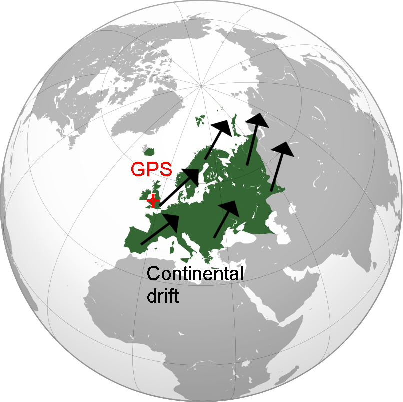
Once you have GPS coordinates, you could either put the GPS coordinates or the local mapping grid positions into your survey data files. The bottom line; cave positions should be given relative to a local grid (or local ellipsoid), not GPS coordinates. And not only because it allows you to combine with surveys that were done using traditional methods.
GPS positions are given relative to a point that is regularly adjusted to remain static compared with the Earth's centre of mass. Continental drift slowly moves all countries and continents around compared with that point. A cave entrance located at 51.8840136123,-3.4364538123 - within Europe - in 2020 would move about 1 metre away within the next 40 years, which can make it awkward to combine surveys whose entrances were fixed to a GPS coordinate in very different years. How important this is depends on how accurately the locations were fixed in the first place, how accurate the surveys are intended to be, and whether the surveys pass close to each other. The amount of motion is different in each continent. In Australia, the motion is about 3.2 metres in 40 years (8 cm per year), in South America and India is is about 1.2 metres every 40 years (3 cm per year), in Africa it is 86 cm every 40 years (1.15 cm per year), in Arabia it is about 70 cm in 40 years (1.5-2 cm per year), and in North America, it is similar to Europe, but in the opposite direction. Parts of Japan and China move at 1 cm per year while others move at 1.3 cm in a different direction.
Many GPS/GNSS tools can be used to convert GPS locations to OS grid locations, but it is important to note that almost all of these tools ignore continental drift, and pretend it is not happening. Your standard handheld GPS device will probably work this way if it can show you grid coordinates. Common surveying applications like Survex and Therion also fall into this category. This makes sense for many GNSS applications, because most GNSS devices cannot measure locations more accurately than that anyway. However, with higher accuracy GNSS, and filtered averaging, better accuracy can be obtained, to the point that a 1 metre error can become statistically significant, and unwanted.
When talking about converting coordinates to grid references, this article relates only to the British mapping system, but the problems are the same as you might find in other national mapping systems. Presumably, most of them will have their own equivalent approaches and transformations.
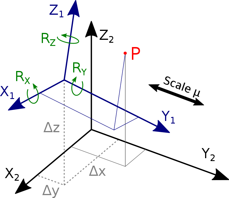
HowToCreate offers a tool to convert from GPS coordinates to "OSGB36" UK grid references using Helmert transformation and transverse Mercator map projection (projecting a part of the Earth's 3D curved surface onto a 2D flat surface). This is only an approximation, using formulas representing the shape of the World used by GPS (WGS84) and the British mapping systems (UK Airy 1830). It is not perfect because the World is not perfectly shaped, and the effects of gravity are not distributed evenly. Points can be displaced up to 3 metres from their actual locations in easting and northing, and that is ignoring continental drift, which can move them further. If transforming altitudes this way, they can be wrong to the point that if you were working on systems spread across a large enough area (100 km or so), groundwater could appear to flow uphill. This only has a fairly small affect on real cave surveys and it can be done quickly with mathematics, so this is the normal approach that is used by lower grade surveys. The cave will be slightly displaced from its true grid reference, but many surveys are already inaccurate enough that a few metres displacement is not the dominating error when comparing caves.
The apparent benefit of using this approach is that when you export a survey using Survex or Therion on most systems (but not all; more on that later) to a format like KML, it will end up back in the same position it was recorded in, because Survex and Therion both use Helmert transformations by default when exporting; when two applications use the same approximation technique, they appear to be doing the right thing, even though it is still an approximation. That position is also what a common phone GPS/GNSS app is likely to produce, because most will work using Helmert transformations. Some better GNSS devices will use better transformation methods though, and will give the correct positions rather than an approximation. The bad part is that the position is technically wrong (potentially by a few metres, but typically less), and coordinates that are exported to GPS using Helmert transformations will become more wrong as time goes on, even if they appear to be correct for a while after they are taken, when converted back using a tool that also uses Helmert transformations. Location data transformed in this way has an error that is not seen in data which is transformed using more capable tools, or via surveying from fixed mapping locations (trigpoints), and that can cause issues when combining high accuracy surveys.
To get the height above sea level (Ordnance Datum Newlyn), you will need to use the Ordnance Survey coordinate transformation tool, supply the GPS coordinates and altitude (pretend they are in ETRS89), and use the National Grid height it returns. GPS altitudes are not directly related to OS altitudes, so simple Helmert transformations (which can also transform altitudes to ellipsoid height) do not give good enough results here; it is best to use actual OS altitudes.
Note that some devices try to show you local altitudes, using Helmert transformation or by augmenting using a geoid model. If so, that will need to be transformed back to a GPS altitude before being converted properly using the OS tools (unless the device is known to use OSTN15 transformation). A real WGS84 GPS altitude is normally about 50 metres higher than the altitudes given by OS mapping (the exact amount varies across the whole country, between 44 metres in Norfolk and 58 metres in the Outer Hebrides). If you do not know which approach your device used to transform the altitude, or you cannot find a tool to convert it back, then do not use that device for locating cave surveys.
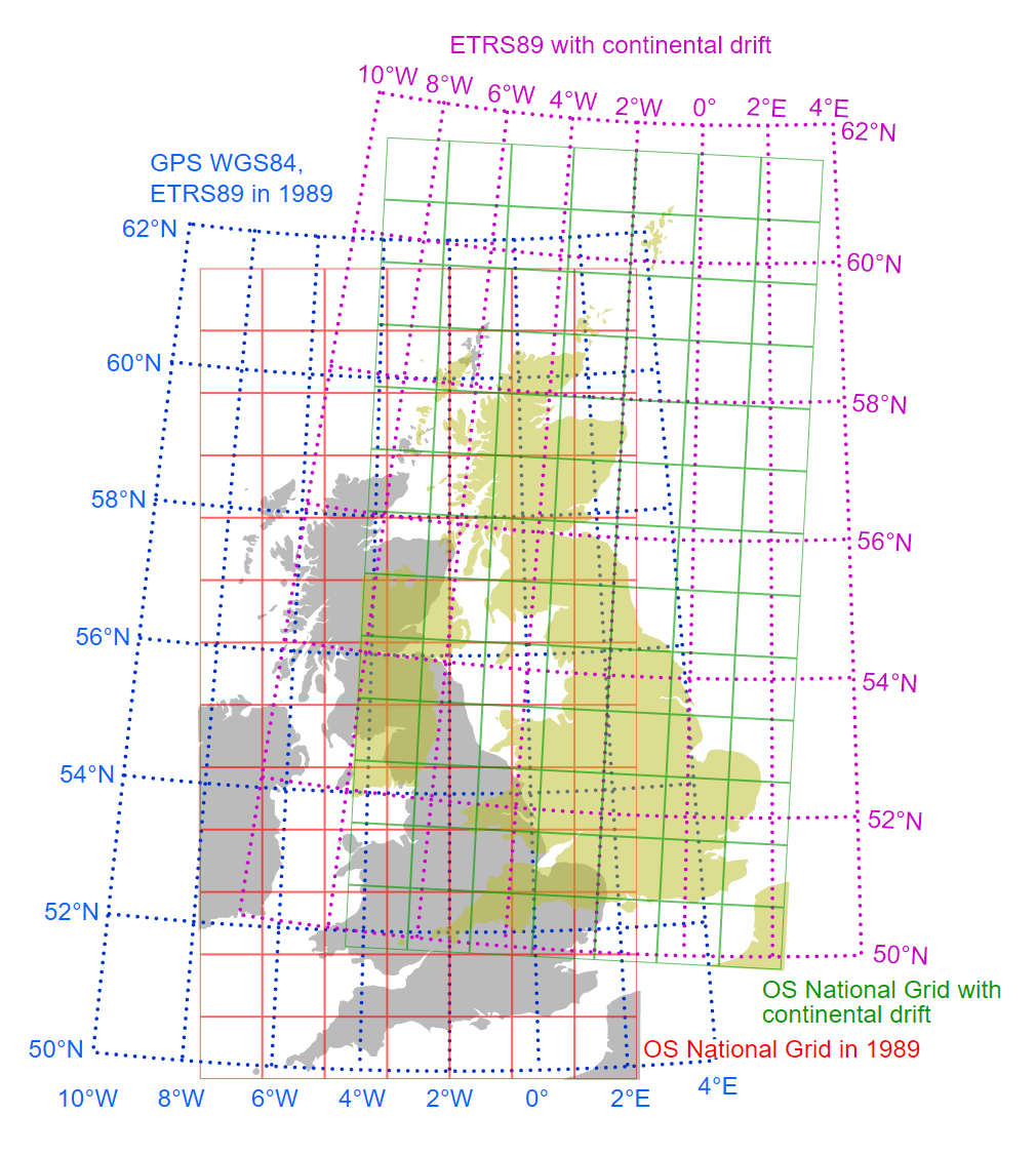
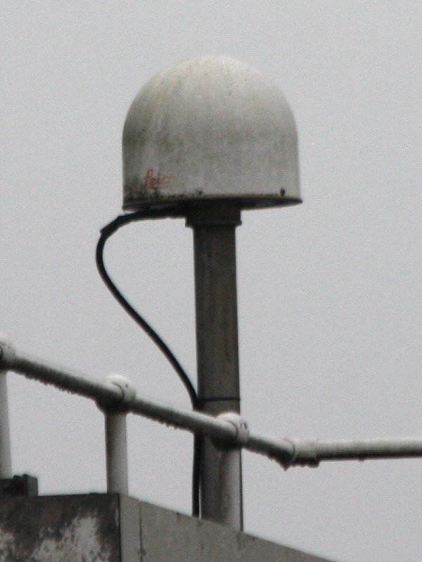
Continental drift moves continents with respect to their GPS coordinates. The speed of this movement is fairly constant, but the fine details are recalculated every few years (known as a "realisation"), to provide better and better predictions of exactly how fast the movement is. To make it easier to use their own GNSS to make maps of the country, most countries use a version of GPS coordinates that are tied to their continents, so the coordinates do not change as the continent moves. GPS uses a model of the Earth and coordinate datum called WGS84. Europe uses one called ETRS89, whose coordinates are based on the WGS84 coordinates from 1989, like a snapshot of GPS, frozen in time. The grid reference you get using a Helmert transformation actually assumes that you are working in 1989. This difference is 79 cm in 2020, increasing by 2.5 cm each year or 1 metre every 40 years. North America has a similar system called NAD83, while Australia has one called GDA94.
To get from GPS's WGS84 to ETRS89, you need to know how fast the continent is shifting north-south, east-west, vertically up/down, and rotationally in any axis around which coordinates. You need to know what date your readings were taken, and what date the target mapping system is based on. You also need to know which realisations are used for GPS and the target mapping system.
This all sounds very complicated - and it is - but it can be simplified with a few steps, and some details. Firstly, in 2020 GPS's WGS84 uses a realisation called IETF2014 (they have ignored a few updates since then, but presumably will change at some point in future). Secondly, the British OS maps are based on ETRS89's realisation ETRF97, as it would have been on 2009.756 (that is 0.756 of the way through 2009, or 00:00:00 on 04/10/2009) - known as its epoch. The coordinates are still what they would have been in 1989, but transforming with an output epoch of 2009.756 causes all of the imperfections in the transformation formulas to be ironed out, to put the coordinates in the right place. You do not have to remember why this happens, all you need to know is that 2009.756 is the epoch used when transforming coordinates into ETRS89 for mapping purposes in Britain. GPS coordinates shift steadily over time, and the epoch of GPS coordinates is <date that they were taken>. Those numbers will all become useful in the following steps.
Differential/relative GNSS systems may output coordinates in either WGS84 or a local one like ETRS89, and you would need to check what yours will output. In Europe, it is normal for differential GNSS systems to output ETRS89 coordinates when using NRTK, which is very useful, because they can be converted directly into a precise grid reference, and you do not need to take account of continental drift when performing the conversions. However, some devices will output their coordinates in WGS84, others can be switched from one to another on the fly (such as the Trimble Catalyst), and some devices can be configured to output their coordinates in one or the other, using post-processing to convert them. Some may allow you to select ITRF2014, which can be considered equivalent to the current WGS84 update (G1762) as long as it outputs it in the current epoch, or they may allow you to select ETRF<number>, which is an ETRS89 reference frame so the coordinates will be in ETRS89.
In reality, each GNSS constellation gives its satellite positions in its own reference frame; they use their own slightly different model of the Earth's size, and their own idea of where "0°" longitude should be according to continental drift, and some even use a slightly different system of telling the time. A device that uses more than one has to perform some complex transformations to get the coordinates from one frame into another, so that it can use the two unrelated constellations together. You do not need to know how all that works, but you do need to know if your device outputs coordinates in a less common reference frame. Almost all basic GNSS devices will use GPS's WGS84, even if they use satellite augmentation, so if it does not tell you what it is using, it is probably that; great, you can skip the rest of this section!
WGS84's latest update to G1762 matches ITRS's ITRF2014 as it would have been in 2010, with predicted tectonic motion since then. It gets updated every year to check that the NGA calibration ground stations (the ones that tell the satellites their actual positions) have got their own positions correct - their coordinates are specified in ITRF2014. The intention is that ITRF2014 (at current epoch) and WGS84 G1762 can be considered equivalent since the stations use ITRF2014 coordinates. High accuracy differential GNSS systems such as the Trimble Catalyst therefore treat WGS84 G1762 as being identical to ETRF2014 at the current epoch. GLONASS uses PZ-90, which was originally up to 15 metres different from WGS84 with an average of 5 metres difference. However, its latest update is almost identical to ITRF2008 (and therefore also ITRF2014), with just a 4 mm difference that needs a very small transformation to get it into ITRF2014. Devices that only use GLONASS might output their coordinates directly in PZ-90. Galileo uses GTRF, which is based on ITRF2014, but is up to 3 cm different from it in some places (because the Galileo project measured those areas more accurately). Devices that ony use Galileo might output their coordinates directly in GTRF instead of ITRF2014, and need to be transformed into ITRF2014 to remove the difference. BeiDou uses CGCS, which can be translated into ITRF97 then transformed through several steps to get to ITRF2014, but the practical difference from ITRF2014 is supposed to be under a millimetre. Devices designed only for BeiDou are likely to output coordinates in CGCS. If needed, there are tools that can convert between the different reference frames of each constellation, but the differences are so small they can be ignored in most cases.
In reality, the actual difference varies more based on how well the ground stations for each constellation keep the satellites updated with their real positions compared with that of the Earth's centre of mass and 0° longitude (which has to stay still according to the Earth's mass, while the continents move around it). The actual differences vary over time, but a 2019 study showed that the practical error in GPS satellites was measured at 1.05 cm horizontally and 3.3 cm vertically, with a 1.77 cm standard deviation. The GLONASS error was measured at 1.76 cm horizontally 5.4 cm vertically, with a 2.78 cm standard deviation. The Galileo error was measured as just 3.5 mm horizontally and 1 cm vertically, with a standard deviation of just 1.6 mm. The BeiDou error for older satellites was measured at 5.05 cm horizontally and 15.6 cm vertically, with a 3.52 cm standard deviation, a fairly substantial error. For newer satellites, the error was measured as 1.27 cm horizontally and 3.9 cm vertically, with a 1.44 cm standard deviation. BeiDou has some accuracy issues as it does not model plate tectonics very well, and is often ignored by high accuracy devices for that reason. A differential GNSS does not have to worry about any of these errors because they will all be corrected by the base station, and the same can be done with post processing. Nevertheless, whichever of these systems a basic GNSS device uses, whether it uses WGS84, PZ-90, GTRF or CGCS, and even considering the errors of that constellation, the output coordinates can be considered to be the same as WGS84, especially given the accuracy limitations of most GNSS devices. Therefore, unless those last few cm of possible error are a problem for you, pretend that all GNSS devices use WGS84, and pretend that WGS84 and ITRF2014 (at current epoch) are the same. However, ETRS89 and WGS84/ITRF2014 should be considered different, because continental drift is an increasingly large problem that can actually be dealt with, and which is already much more significant than the differences between the constellations.
Note that within China, authorised devices are also likely to apply an obfuscation known as GCJ-02 which adds random offsets to the standard GNSS coordinates, to give coordinates used by the national mapping system. This offset averages 300-500 metres, and is by far the overriding source of error within China. The most popular online mapping service - confusingly called Baidou - adds a second layer of obfuscation. This page caters only to standard coordinate systems used elsewhere, and does not cater to the Chinese mapping system.
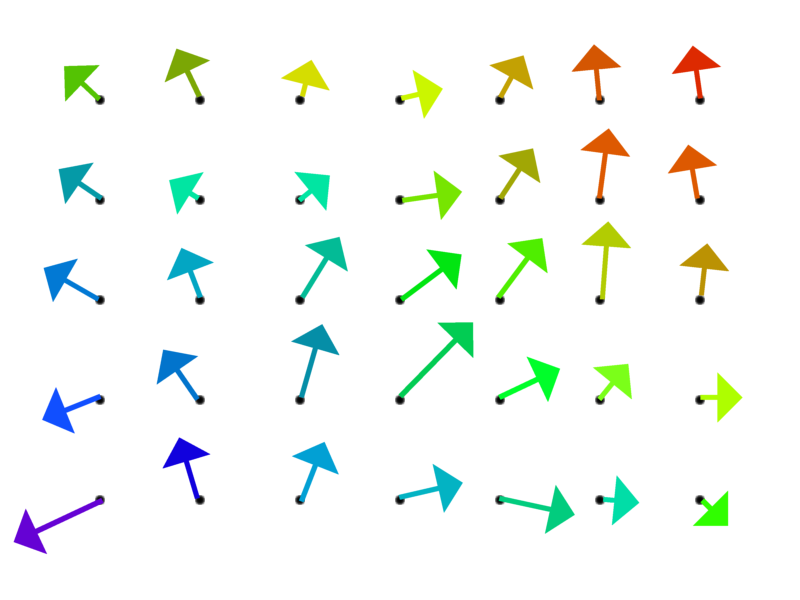
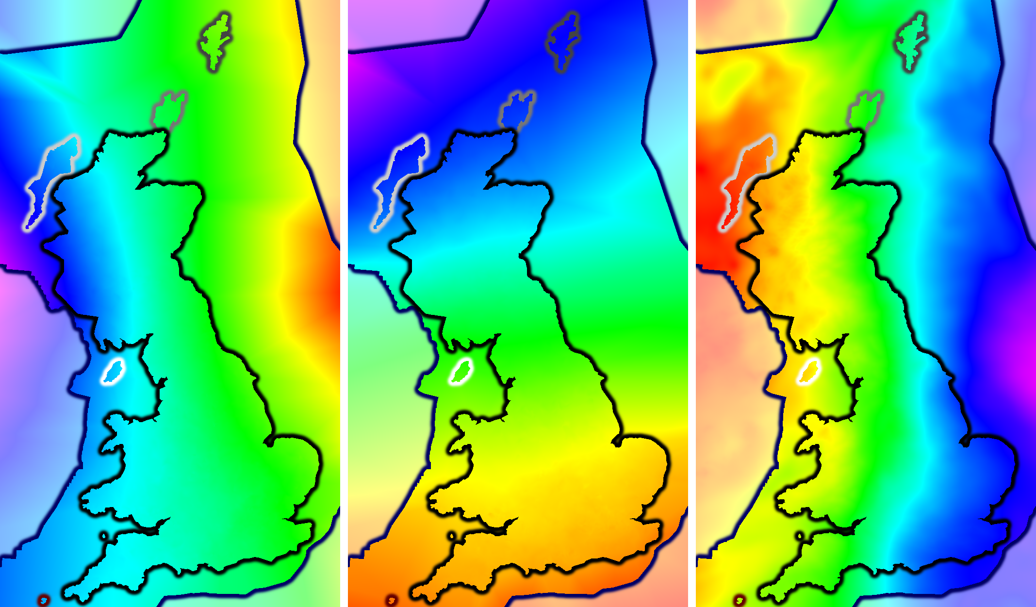
The UK Airy 1830 earth model is still a very good representation of the Earth under Great Britain, and it is still used by most simplistic transformation tools with a basic Helmert tranformation. However, it is not perfect. Gravity is not so regular, and across the whole island, it has inconsistent effects. The Ordnance Survey use a rubber sheet transformation when converting from ETRS89 coordinates to grid references. This takes into account all of the variances around the UK. For every kilometre square, they use a specifically shifted earth model that more closely matches the effects of gravity at that point on the Earth. Each of them is based on the ETRS89 earth model with a manual shift into Airy1830, but tweaked slightly to match that particular area. They call this model of the Earth OSGM15 (that's the vertical part), and the transformation formulas which use it OSTN15 (that's the horizontal part). OSTN15 also takes into account the distortions of the old mapping coordinate system, so that the old grid referenes can remain in use, without needing to correct the 20 metre error over the length of Great Britain. This gives a much more accurate coordinate shift, so that the conversion to OS grid reference and altitude is now perfect. (The actual expected accuracy of OSGM15 is 8 mm, and OSTN15 is 0.0000005%, or 5mm across the length of Great Britain, but it is the fundamental model used by British mapping, so it is treated as if it has no error.)
An eastwards shift is always expected since the Airy 1830 ellipsoid datum used by British maps is situated about 100 metres west of the ETRS89 datum; to put that in other words, the 0° lines on the two earth models are located about 100 metres apart in Greenwich. A graduated southwards shift is also expected because the Airy 1830 earth model is smaller than the GRS80 earth model used by ETRS89, and it is pulled closer to the actual surface. But localised differences, or differences between the east and west coasts, reflect the changes in gravity.
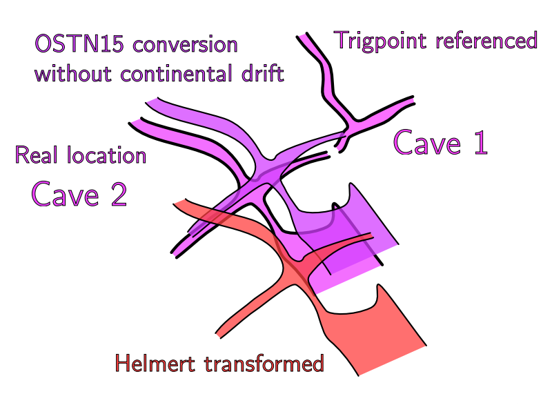
Survex and Therion use the underlying "PROJ" utility to convert coordinates. It is possible to make PROJ use the more accurate OSTN15 conversions on some systems. When this happens, Survex and Therion - depending on whether they were compiled to use the resources of that system - might then give different coordinates from what they would give on a system that has not been prepared that way. Two computers can give two different results, for the same survey. This is not particularly helpful unless you can ensure that the survey is only compiled on a system that has been prepared that way.
There is he hope that in future, PROJ might be updated to always use OSTN15, on all systems. The problem with this is that it would need to be precompiled on Windows (normally) and would therefore need to include the enormous OSTN15 database as part of the installer; not impossible. This only solves the gravitational distortions part of the problem, but fails to account for continental drift. Solving that part would require PROJ to apply continental drift, automatically detecting the continental plate and how much drift to apply based on the coordinates, and then convert it to the correct reference frame for the mapping used by the relevant country. This is not impossible (there are external tools that can do it), but it is asking a lot from the PROJ project to implement this for the purpose of cave surveying.
There is some value in keeping a record of the original GPS coordinates, and how accurately they were converted, but that should be done as a comment. There is very little to be gained from leaving the coordinates at their original WGS84 values, and hoping that at some point in future it might be possible for Survex and Therion to use the coordinates, coordinate system and date to apply the correct continental drift for that location, and then apply OSTN15 to convert the coordinates into the British OSGB36 grid. Long before that happens, your survey would have been published, with the wrong coordinates, which everyone will have started using. The coordinates would then randomly change at some point in future, probably inconsistently on different systems, depending on how much had been implemented at that time. Inconsistent results would happen right away, depending on how the PROJ utility had been installed.
It is far, far better to convert it, accurately, once and for all, and use the converted coordinates. Then no matter what date someone compiled the survey, no matter what system they use, no matter what version of PROJ is installed, it will always use those correct coordinates. Consistent and accurate.
This is the recommended approach, particularly for high accuracy surveys. To simplify the process, I have released a High Accuracy WGS84 GPS To British OSGB36 Grid Reference Conversion tool, that performs the required conversion steps and calculations in the right order. Assuming it works, you can just use that. Enjoy!
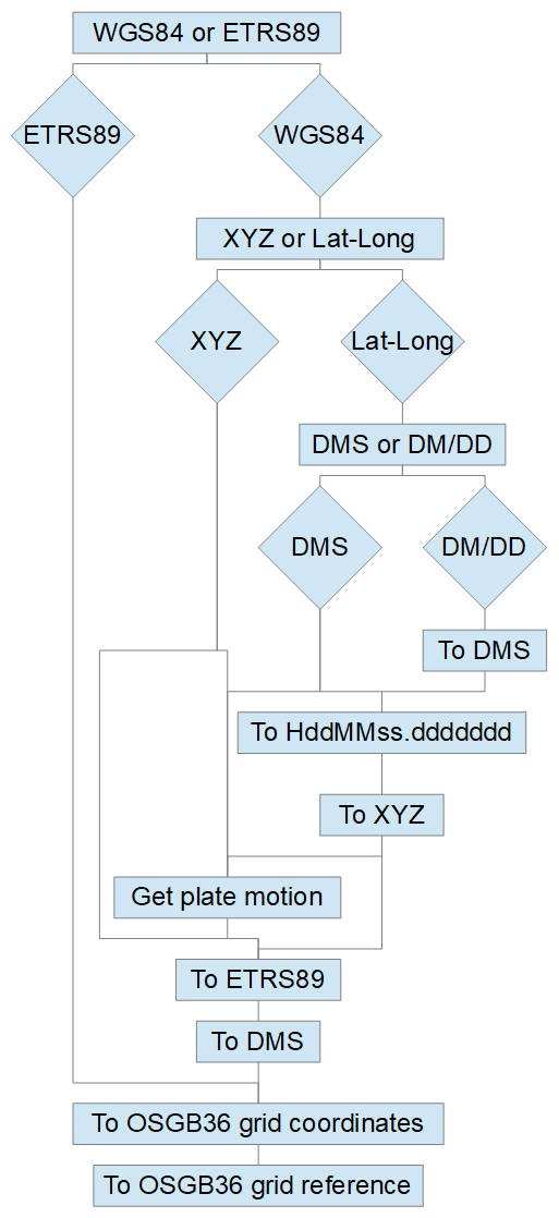
Conversion relies on some external tools, and as a result, it is possible that it could stop working in future, if those tools ever go offline. If they ever go offline, you would need to manually perform the steps instead.
Manual conversion is done using a series of tools, though most of the steps can be automated using the HowToCreate library (all except the continental drift measurements), if you would ever like to implement it yourself. Imagine that the GPS coordinates start as 51.8840136123,-3.4364538123,938.946 - if your GNSS device (such as a differential GNSS) exported these as ETRS89 coordinates, you can skip the 6 steps below.
Your coordinates have now been converted from WGS84 to ETRS89, in the correct epoch for OS maps. Unfortunately, most cave surveying software, such as Survex and Therion, do not have a way to tell them that the coordinates are specified in ETRS89. You can only say that they are in WGS84, which is not correct. So you need to convert them to grid references. At this point you could just use the HowToCreate tool to convert from GPS coordinates to UK grid references using Helmert transformation (SO 01227.8516 21580.8193), and just use the Ordnance Survey coordinate transformation tool to get the National Grid height. Once again, Helmert transformations are only an approximation, with all of its ≤3 metre inaccuracies. It matches what Survex and Therion will export, but now as ETRS89 coordinates, not the original WGS84 GPS coordinates. The good part is that it would give the same results for the equivalent GPS positioning, no matter what year you take your readings, and no matter how far the continents have drifted. Maybe that is enough for you. The bad part is that it is not actually the correct grid reference, even if some other tools agree with it because they use the same approximation.
However, at this point, you have already made something that does not convert back to the original GPS coordinates when exporting from common tools. (And it really shouldn't convert back to the same coordinates in tools that understand continental drift, because continental drift will change those coordinates over time.) It is technically as perfect as you can make it, so you may want to keep it perfect, and apply the OSTN15 transformation to get the true grid reference for your GPS coordinates - the same one that the Ordnance Survey would give. Use the Ordnance Survey coordinate transformation tool, supply your ETRS89 coordinates and altitude, and use the Easting, Northing and height it returns (eg. 301228.543 221580.168 886.000). You can now use the HowToCreate tool to convert it from UK grid coordinates (301228.543,221580.168 - note the comma) to UK grid reference (SO 01228.543 21580.168). Note that if you are using the Ordnance Survey coordinate transformation tool to get the grid reference, you can skip step 6 above, and just supply the X,Y,Z ETRS89 coordinates directly to the tool.
At this point, you have the best possible OSGB36 grid reference, compatible with the OS grid. Your coordinates have been converted in a way that the OS refer to as "error free"; your GNSS positioning can have errors, but the conversion does not add any more. If anyone is using a high quality GNSS that understands continental drift or works in ETRS89, and is aware of OSTN15, and they supply it with your grid reference, it will take them to the correct location. If someone uses a GNSS device that does not understand continental drift or OSTN15, it will get them close enough to locate the entrance; within 4 metres of it in 2020 (well within the accuracy of most GNSS devices) - over time, the error caused by their GNSS device's conversion routines will slowly increase by 1 metre every 40 years, but the same would happen if you just supplied them with the original GPS coordinates. It is the device's conversion routines that are adding errors here, not yours. But most importantly from a surveying perspective, if another cave nearby is surveyed to the same accuracy, with the right conversions, the only errors in the positioning will be in the accuracy of the readings that are taken from the surveying tools, and the caves can be compared as if they were surveyed as part of the same project. Continental drift will not affect the positions, and water will continue to flow downhill. The cave location will be compatible with any other cave surveys whose entrances were located using a benchmark, trigpoint, or OS map, which is how they were all done before GNSS took over.
Just a note; you may be wondering why the conversion uses 2009.756 as the output date, when ETRS89 coordinates should not change over time. This is because each stage of the ITRF2014 to ETRS89 conversion is performed using Helmert transformations from one frame to the next. These transformations are imperfect (but extremely good!), so each little update has a set of little corrections that it applies when transforming from the previous one. Ordnance Survey have determined that frame ETRF97, pushed to epoch 2009.756, provides the best set of transformation corrections, and puts the coordinates in the right place over the relevant part of the continent.
This requires an extra step. The UNAVCO Plate Motion Calculator produces the plate velocities for the plates in relation to WGS84, which is the direction needed to get from WGS84 to ETRS89. There is no equivalent tool to provide the plate velocities in ETRS89, and it is not as simple as changing some numbers. However, the correct numbers would have been given as part of the answer in step 5 above. Those were the three numbers at the end of the result that were ignored. So there is a catch 22; you need to have gone from GPS WGS84 to ETRS89, in order to have the numbers needed to go back from ETRS89 to GPS WGS84.
All is not lost. You can pretend that your ETRS89 coordinates are WGS84 coordinates. Use them to get the plate motion velocities. This can get the wrong result if your ETRS89 coordinates are immediately northeast of a tectonic plate boundary (within the amount that continental drift has moved ETRS89) - this matters in Iceland's Thingvellir National Park, but not in Great Britain. It can get the tiniest error if your coordinates are right next to a place where the plate motion (which is supplied at 0.01 mm precision) was about to change by 0.01 mm in any of the directions. This has no practical effect in real cases; your end result may be wrong by a fraction of a millimetre, but that could just as easily happen because of the plate velocity precision anyway.
You can then put the numbers into the EUREF ETRF/ITRF Transformation tool, as if you were transforming from GPS WGS84 (ITRF) to ETRS89 (ETRF) - the wrong direction. It will give you a result containing the three numbers that you need to convert in the opposite direction.
You may notice tiny differences when converting backwards and forwards, which are caused by the precision limitations of the tools used. The example coordinates above, when converted back again using this approach, give an error of just under 0.5 mm, most of which was caused by the OS tools truncating grid reference precision to 1 mm. That is well within the limitations of cave surveying anyway.
Some trivia for the mathematically inclined; there is actually a mathematical solution to the problem of having to use the plate velocities at the wrong coordinates. Check the forward shift at the new point, and if it does not match the original point, apply the reverse shifts computed at the new point to the original point and try again, iterating until the change in reverse shift parameters is within a nominal threshold like 0.01 mm. In this case that is not worth it, because that is already the maximum likely error after the first try anyway. Also, the conversion tools have already limited precision to a larger margin than the error anyway, so the tiny 0.01 mm potential error would be drowned out by the precision limitation. Iteration like this is actually used in three other steps of the conversion; once for reversing the OSTN15 bilinear interpolation, once for reversing the transverse mercator projection, and once for converting cartesian coordinates to geodesic.
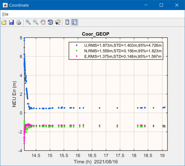
If you wanted to give RINEX PPP or PPK a try from a consumer-grade product (excellent choice!), use the RINEX export feature of your device if it has one, or the Geo++ RINEX Logger app on Android (if this app keeps showing a "Please wait" screen, then your device cannot be used to export RINEX data). Record in static (not kinematic) mode, if your device lets you choose. It can be important to know what satellite constellations and frequencies your device supports, so check for this information in its instructions, settings or in its satellite overview.
Android devices will try to save power by randomly sleeping the GNSS chip, especially while the screen is off, so no data will be gathered for substantial parts of the capture time. It also will only allow a foreground app to continuously access the GNSS raw data, even if the app is allowed to access data in the background. In the Android app permissions, you will need to ensure that the app is allowed to access the position even when running in the background, just in case some other app steals the focus. In the Android app settings, ensure that Android does not optimise battery usage for that app (so it doesn't close it automatically when it thinks you are not using it). In the Android battery settings, ensure that it never puts that app to sleep. You will also need to tell Android 9+ not to sleep the GNSS chip randomly after a few seconds of use (known as duty cycling). Enable Developer options; in Android settings go to "About phone - Software information" and tap 7 times on "Build number". Go back to the settings page, then into "Developer options" and enable "Force full GNSS measurements". Most importantly, keep your screen on at all times; you will probably need to install an app like Awaker, since most Android devices do not let you choose to keep your screen on forever. You will probably need an external battery pack. Keep the RINEX logging app focused at all times - do not be tempted to switch to another app while logging. Disable phone and data connections to prevent notifications from other apps from stealing the focus. Android devices are a very frustrating way to gather RINEX data. Keep your eye on system updates, because no doubt there will be some other change that breaks it again in some other secret way, and you will need to go hunting for whatever secret option might make it work properly again, or the options you rely on now might just disappear like many other location settings have in the past. On Android, the GPSTest app from barbeauDev can show what constellations and frequencies your device can see, and Geo++ RINEX Logger can tell you what constellations and frequencies it actually recorded.
It is perhaps worth noting that Android does not natively export RINEX data. Instead, it exposes some APIs which export different pieces of the data, not in RINEX format. The app has to take all these separate APIs and use them to construct a RINEX file itself. The version of the operating system makes a difference as to how much data can be collected. Android 7 was the first version that could collect useful data, and Android 8 was the first to expose dual frequency and carrier frequency. The quality of the app also makes a big difference. Geo++ Rinex Logger has the longest history, and a large amount of testing, and is generally the recommended app. While there are many other apps, they do not all log the same amount of data, or the same quality of data. Devices only started exposing carrier frequency information in 2018.
Most freely available data files are delivered in one file per day. While the tools can process times longer than that, or a directory of files, Net_Diff cannot cope with multiple base station files. If you wanted to do captures that are longer than 24 hours, you might have to combine them into one, or you might need to tell the tools to only process a subset of the capture within one day. So to keep the process as simple as possible, start and end your captures within the same GNSS day. A GNSS "day" starts at 00:00:00 UTC (GMT), and ends at 23:59:59 UTC. Your clocks will need to be all perfectly synchronised to work at the limits of that time, so it is best to start and end recording some time well within those times.
Export the resulting file to a computer (typically named [something][day_number].[year]o). If it created multiple sequential files, you will need to append them to make a single file (see the section on obtaining files below). Note that some devices record much more satellite data than others; a Garmin GPSMAP 66sr records about 42 MB over the course of 5 hours, while Geo++ RINEX Logger on a Samsung Galaxy S20+ records less than 5 MB in the same time, due to the system randomly deciding not to allow it to access the GNSS raw data. After forcing the system not to duty cycle the GNSS chip, it gathers 42 MB. However, until the Garmin GPSMAP 66sr has an update to fix the loss of satellite visibility after 3-9 hours, it will not be possible to use it reliably for more lengthy captures. The results from a device that gathers more data can be substantially better for PPP or PPK.
There are a number of applications that can perform PPP or PPK. The most popular one is RTKLIB, but the Net_Diff application seems to get far better results. RTKLIB is far more easy to understand, and has plenty of tutorials. Net_Diff has a complex UI that is initially challenging to use, but its instructions can help, and the steps given below should be enough to get it working. Net_Diff is recommended because in testing, it refined positions to within just a few centimetres, while RTKLIB would get about a 1 metre error in the best case when using the same data. Selecting the wrong options in RTKLIB added a number of metres to the error with no obvious indication of which options gave the best accuracy. Net_Diff can also download supporting files for you, which is a major benefit.
Whichever application you choose to use, it is usually possible to use either ephemeris data usually delivered in files called "brdm*" or "brdc*", or the much more accurate orbit ("*.sp3") and clock ("*.clk") files. For best results, wait for at least 12 hours after taking the readings, so that the updated sp3 and clk files can be made available. These can be downloaded from a number of different sources, and may contain the data measured from any number of observation stations. Some supply the details of more satellites than others; recommendations are given below. If you are using a separate base station (in addition to a CORS base station) and rover, or if you have a high quality device, your device may also export a separate "*.nav" file, which can also be used in place of the broadcast ephemeris and clock files. In personal testing using Net_Diff with a 10 hour RINEX log from an ArduSimple RTK Calibrated Surveyor Kit, the results of the last 5 hours of processed data with a "*.nav" file gave a calculated position just 0.5 mm away from the same portion of the data when using the accurate orbit and clock files. Those were both within 6 mm of the position calculated using a Trimble Catalyst in NRTK mode. High quality devices definitely get better results than low quality ones, and the "*.nav" file results can be excellent for longer captures with those devices.
As for whether to use PPP or PPK, that part is really up to you. PPP will give results in WGS84, which needs continental drift conversion to get it into local grid correctly (the HowToCreate High Accuracy conversion tool can do this for you in Great Britain). PPK will give results in whatever reference frame the base station is set up for; ETRS89 for the OS Net base stations (again, the HowToCreate tool can do the grid conversion for you). They each get good results, with a similar amount of error. PPK seems to give less variance over time, and is definitely very effective, good results can be obtained with as little as 2 hours of data (though 5 is suggested). PPP - when performed with Net_Diff - is extremely effective too, but needs a little longer time to get high accuracy. PPP does seem to get higher precision than PPK over time, as in the end it might only get a few millimetres of jitter, but this needs long observation times. PPK, meanwhile, after initially settling down, often never gets much more precise than it originally was, but that is because it is extremely precise already. However, when using PPK with a high quality device, the occasional jitters can be seen to slowly reduce over the first few hours; with an ArduSimple RTK Calibrated Surveyor Kit, the jitter reduced to less than half a millimetre after 5 hours, so a 10 hour capture was used to refine the position even further. PPK is suggested as being the better option, if you have data from a nearby base station to use for it.
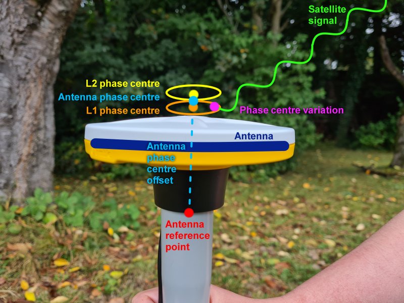
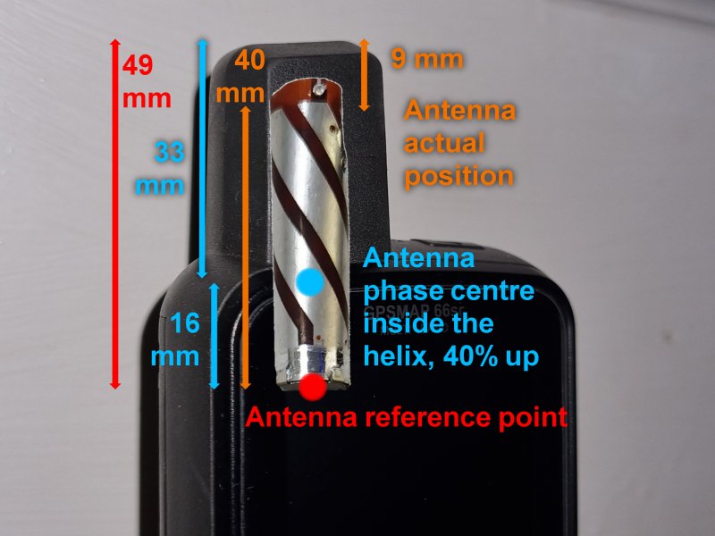
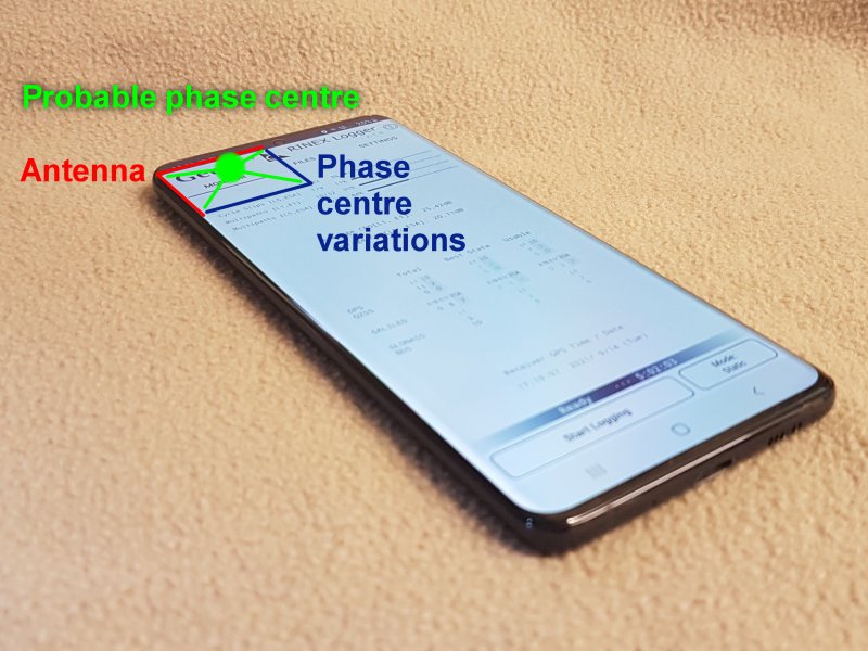
GNSS devices measure the position of a point outside their antenna, which is not normally a physical point on the device. With PPP or PPK, you will need to subtract a number from the resulting height, to get the height of the point that you want, such as the base of the device or tip of the antenna. With PPK, you will need to add on the height of the base station's equivalent offset too, or you can end up with a significant error in the height. This means you will need to find out the offset for both your device, and the base station you are using. The two devices are likely to have very different offsets, and they will not cancel each other out. The good part is that if you are using Net_Diff, and you are using a common professional grade antenna, and your base station is also using a common professional grade antenna, then you don't have to read this section at all, because Net_Diff already compensates for the antennae for you. However, you will need to read this part if you are using an uncommon or non-professional antenna such as a handheld device, or if your base station uses an unusual antenna, or if you are using RTKLIB.
Due to the physics of how electromagnetic signals induce electrical charges inside an antenna, and the interference of the waves as they interact with the parts of the antenna (called an equiphase wavefront), the GNSS device will end up seeing the signals as they would have been at some position slightly outside the antenna itself, known as the antenna phase centre (APC). Think of it like the focusing point for a lens, where all the beams cross. When a GNSS device calculates a position, this is the position it is actually calculating, and this is also the point whose coordinates the post processing will be calculating.
Different shaped antennae have their phase centres in completely different positions. For flat or cup-shaped antennae like most high accuracy devices use, the point is actually slightly above the antenna. The antenna must be kept perfectly vertical (away from the Earth's centre of mass) since otherwise you can shift the phase centre sideways, and the maths gets much harder. For most helical antennae like low end handheld devices use, the point is inside the centre of the helix, normally about 40% of the way up the antenna, but this can vary depending on the design. At the accuracy level required to locate a survey for most cave surveying work, the standard offset supplied by a manufacturer can be used, but manufacturers of basic GNSS devices are very unlikely to supply details of the phase centre of the device, so an approximation may need to be made. The common length of a helical antenna is 4 cm (about a fifth of the GNSS wavelengths), part of which may be buried inside the device. In a 4 cm helical antenna, the average antenna phase centre will be about 1.6 cm up the antenna - the electrically receptive parts of it, ignoring any housing. With a phone, the GNSS antenna is often somewhere near the top corner on the opposite side from the camera (you may be able to find schematics for your device showing its location). The phase centre is typically within a 3 cm square from that corner of the phone, presumably sitting just above the surface of the screen (usually 1-2 cm above the device) when the phone is lying on its back. This is information a phone manufacturer will never provide, and it is different with each design, but it really doesn't matter at this accuracy level unless you manage to do some extremely precise post processing.
Nerdy details paragraph. The exact position of the phase centre varies slightly with the frequency of the signal (so L1, L2 and L5 signals all have slightly different positions that they will appear to be focused, compared with the antenna, with L2 and L5 higher up than L1). The phase centre is actually different for satellites at different angles, as their waves interact on a slant over the antenna surface. These get a phase centre variation (PCV) of a few degrees. The general approach is to take the average of all the phase centres, for satellites at all angles, and use that average as the phase centre. On a high quality base station antenna, the phase centre will normally be only slightly offset horizontally compared with the actual centre of the antenna, on the order of 0.1 mm. The biggest difference will be vertical, where the phase centre is usually a few centimetres above the antenna plate itself. Highly precise industrial post processing software allows you to supply all of these numbers separately; the phase centre offsets in the northwards, eastwards and vertical directions, for both L1 and L2 - and yes, you are supposed to orient one specific side of the antenna northwards for that. Due to manufacturing imperfections in the antenna, each device will have a slightly different point, even if they are the same model number. The difference between two identical devices might be in the order of 1-2 mm. For even more precise work, the phase offsets for the specific antenna would need to be measured precisely in a laboratory setting; this is done for base stations that need to be positioned accurately within millimetres. For even more precision, the angle of each satellite could be modelled separately, so that the PCV adjustment could be made to each separate signal. This could either be the generic numbers for a typical antenna of that model (this is what Net_Diff does), or the specific calibration is measured for the specific antenna. This is useful for setting up a permanent base station like the OS Net CORS base station, where you might want 0.1 mm accuracy. Cave surveys do not need this level of accuracy!
For the simple post processing covered here, the basic average antenna phase centre offset (PCO) is needed, and that is all. The offset is the distance from the nominal antenna reference point (ARP) of the device, to the phase centre - the real measuring point of the device. The normal ARP of a flat dish antenna will be the base of the device, where you screw it onto a tripod or pole, but you need to check the details for your specific device. When using a professional GNSS device in its normal operation mode, it will normally subtract this for you, so that the heights it gives are for the reference point, not the phase centre. However, for post processing, you need to take care of this yourself, unless your post processing application can do it automatically for you.
In the case of a device with an antenna phase centre that is about 3.3 cm below the tip of an upright antenna (such as the Garmin GPSMAP 66sr), assuming you want your measurements to be taken from the centre of the tip of the antenna, your phase centre offset will be -0.033 metres. This means you will be subtracting a negative number from your results, and the height of the tip of the antenna will therefore be 3.3 cm higher than the result that post processing gives you.
For PPK, the corrections are relative to the base station's phase centre, not its antenna reference point. The base station RINEX file will contain the position of the base station, but this position will normally be the antenna reference point of the device, not the actual phase centre (since that will be different at different frequencies). Also in that RINEX file, it will normally tell you the antenna model on a line ending with "ANT # / TYPE". You can normally look up the specifications of these antennae to find the phase offset (some post processing software can do this automatically). For example, many OS Net base stations are identified as "LEIAR25 LEIT", which is a Leica AR25 with LEIT radome. Net_Diff knows this specific model, and would already have applied corrections for it, so you would only need to look up the antennae phase centre offset if you are not using Net_Diff. Ordnance Survey publish the standard phase offsets of their antennae. This particular model has a very minimal horizontal offset, but a very significant vertical phase offset from the nominal base; 0.1551 metres for L1 and 0.1631 metres for L2. That is a 15-16 cm vertical error if you fail to handle it correctly. If you are just using single frequency PPK, use the L1 phase centre offset. If you are using dual frequency, Ordnance Survey give a formula to work out the phase centre offset from the two frequency specific phase centre offsets (which ends up being positioned below both the L1 and L2 phase centres). Phase Centre Offset = (2.545 x <L1>) - (1.545 x <L2>), which in the "LEIAR25 LEIT" example would be (2.545 x 0.1551) - (1.545 x 0.1631), which is 0.14274 metres.
So now you have two offsets; the phase centre offset for your device (with a flat dish type antenna, it will be above the antenna reference point, so the number will be positive), and the phase centre offset for the base station. If you want to do this the simplest way, the phase centre offset for the base station gets added to your height, and the phase centre offset for the GNSS device gets subtracted from it. So in the case of a Garmin GPSMAP 66sr using a "LEIAR25 LEIT" OS Net base station, the height of the device gets 0.14274 added to it (if you are not using Net_Diff), then -0.033 metres gets subtracted from it, so the tip of the antenna will actually be 17.5 cm higher than the height that gets calculated by post processing.
This is fine when working with a base station that is close to you (it is imperfect, but the error is less than a millimetre when working with your nearest base station in Great Britain). But when working with one further away, the curvature of the Earth comes into play, because what is "up" for the base station is not exactly "up" for you. For convenience, RTKLIB lets you specify the phase centre offsets for the base station and GNSS device in the options, so you do not have to worry about which way is up.
If you are using some other post processing software that does not let you specify phase centre offsets, and you want to add the base station's antenna phase offset height accurately (rather than ignoring curvature and adding it to the final result), you can use the HowToCreate High Accuracy conversion tool to convert the base station's XYZ coordinates (which are in the base station's RINEX file) into latitude, longitude and height. Manually add the base station's phase centre offset to the height, and then convert back to XYZ. Use these numbers to replace the base station's coordinates that you give to the post processing software. You might also need to do this if you are using Net_Diff, and your base station uses an unknown antenna without any available ATX data.
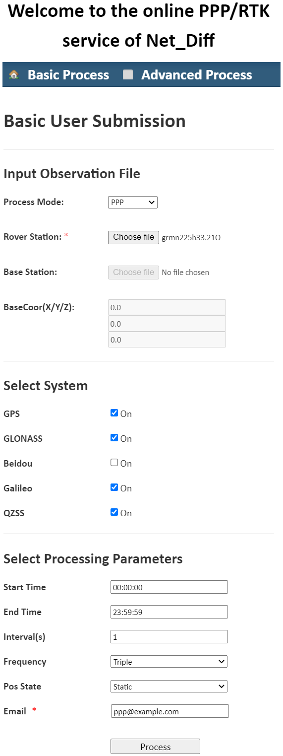
If you want to make life easy for yourself, you can try Net_Diff's online version, operated by a very slow connection from China. This offers much less control, and you have to hope it manages to download a useful set of .sp3 and .clk files, for an observation site that happens to give reliable results. It does seem to get extremely good results for PPP, within a few centimetres horizontally and 15 cm vertically in personal testing with a 5 hour RINEX log. Wait for at least 12 hours after taking the readings so that the external data files it uses can become available. After a full day, better files become available so it can get even better results (it gets a little more accurate a few months later when even more detailed data files are released), select the rinex file your device created, enable the constellations your device supports, say how often your device takes a reading (usually 1 second, check the timestamps in the file), and select triple frequency mode if you want all the possible frequencies to be used. Remember that the antenna phase offset for your device now needs to be subtracted from the results (eg. subtract -0.033 metres for a Garmin GPSMAP 66sr).
Alternatively, the Canadian CSRS-PPP service can also do PPP for free (make sure you select "Static" and "ITRF"), but only works with GPS's L1 and L2 frequencies and a single GLONASS frequency, and ignores GPS's L5 frequency and other constellations. In personal testing, the results are a little better than using averaging, but not as good as Net_Diff, and with some devices the position was completely wrong. Registration is required for CSRS-PPP. Trimble also offer their online Trimble RTX service (registration required), but this relies on the device supporting GPS L1 and L2, not L5. It also needs the device to have a common, professional grade antenna. As a result, it cannot be used with most consumer grade devices, and is evidently aimed at Trimble customers who want to post process the data they obtained from a Trimble device.
If you want to try PPK, you will normally need to use a desktop application such as Net_Diff or RTKLIB, and you will need to download all the files yourself if using RTKLIB. However, the online version of Net_Diff can also perform PPK - you need to supply a nearby base station's file. For dual frequency devices, it needs the device to use GPS's L2 frequency, while some dual frequency devices use GPS's L5 frequency instead, so you may need to treat your device as single frequency. In personal testing with the online version, PPK refined the position very nicely, but never in the correct position. Sometimes it was less than a metre out, while other times it was several metres out, when using the same data. This changed randomly depending on which day the data was uploaded. Exactly what causes this is not known, but the desktop version can be made to give correct results with the same data. The online version is not recommended for PPK.
For PPP or PPK, you will need your device's RINEX file (called an observation file), and either ephemeris files (with RTKLIB you will always need this file), or clk and sp3 files. For PPK, you will also need a base station file. If you are using an ArduSimple device, see the instructions for how to get RINEX out of an ArduSimple device that you also want to be able to use for RTK.
If based in Great Britain, you can use the Ordnance Survey's OS Net base station (CORS) data, but note that the free data has a relatively low sample rate of one per 30 seconds, so longer recording times are needed for accuracy (eg. 30 minutes plus 5 minutes per km from the base station might be enough if you have a high quality GNSS device, but 5 hours is a good start for lower quality devices). If not, you will need to find your country's equivalent. The free data from the OS Net website currently only records GPS and GLONASS, and only the L1 and L2 frequencies, while most dual frequency consumer grade devices use GPS L1 and L5. As a result, when using PPK with that version of the Ordnance Survey free data, only two constellations can be used, and normally only using a single frequency. Nevertheless, the results can be surprisingly good, as the PPK base station data largely replaces the need for dual frequency. The OS Net data available from other sources records GPS L1, L2 and L5, GLONASS G1 and G2, Galileo E1, E5a and E5b (and the E5 midpoint between E5a and E5b), and BeiDou B1, B2 and B3. Wait a few hours for the Ordnance Survey data page to update (it updates on the hour with data 1 hour old, so it can take up to 2 hours before the data you need becomes available), or for the EPOS site to update. For the OS Net website, go to the Ordnance Survey RINEX data page, search for your grid square or GPS coordinates (use their input formats help), and ask for the nearest 1 station, on the date you were testing (which must be less than 45 days ago), for the time range of 0 to 24 hours. The results page should give you one station (if not, correct your mistake and try again). Select that station and download the RINEX data. This should come in a file called [station][day][letter].[year]o.
The EPOS GNSS data gateway site contains data for a lot more base stations around Europe, including the UK base stations, and gives the complete OS Net data for all observed constellations. The OS Net data sometimes takes several days to get added to the site. Sometimes it never appears. Use the map to search for the nearest base station, or search for it by name if you know it. Click on the station. Either click on "Metadata details" in the map balloon, or set the radius to 0 and click on the station name in the table below the map. Click on "Data availability", select the month that you are interested in, select the day that the readings were taken, and click on "Download selected dates". Unzip the downloaded file using a utility like 7-Zip. This should extract a file called [station]_[letter]_[year][day]0000_[days]_[frequency]_[letters].crx. This is a CRX (compact RINEX) file, which needs to be converted into a RINEX file. The RNXCMP crx2rnx utility can do this. Install it into an appropriate directory (just download and extract the relevant zip file), open a command prompt on your computer, and run the command C:\path\to\crx2rnx.exe C:\path\to\the_crx_file.crx (or the equivalent for your system). It will create a new RINEX file in the same directory, with the same name, ending in ".rnx". That is the file you need.
If you have ended up with multiple separate RINEX files because your GNSS device or base station created two for different time spans (eg. Geo++ RINEX Logger creates multiple files per day, and OS Net creates one file per UTC day), you can combine them by appending them into a single file and removing the header from the second file. If the first file has a line ending with "TIME OF LAST OBS" (it will be near the end of the header section), copy the one from the second file into the first file. You can optionally remove any lines ending with "# OF SATELLITES" or "# OF OBS". Alternatively, the gfzrnx utility can be used to combine multiple RINEX files into a single output file. Sometimes, gfzrnx seems to create a RINEX 2 file when appending files, which can lose data if your files started out as RINEX 3. As a result, it helps to be specific. The following commands assume you want RINEX 3, but you can use "::RX2::" instead of "::RX3::" if you actually wanted RINEX 2. You can also use -fout combined.rnx --version_out 3 if you wanted to specify a file name. This command combines two files into a RINEX 3 file: gfzrnx -finp file1.rnx file2.rnx -fout ::RX3::
If you want to use ephemeris data, one of the easiest places to obtain it is the NASA Broadcast ephemeris data page (registration required). Open the "Daily GPS Broadcast Ephemeris Files" directory. From here, choose which files you want to use, based on what constellations you might need to use. For all constellations at once, download the "brdm*" file located in YYYY/DDD/YYp/BRDM00DLR_S_YYYYDDD0000_01D_MN.rnx.gz (eg. for the 286th day of 2020, you would need 2020/286/20p/BRDM00DLR_S_20202860000_01D_MN.rnx.gz). For GPS, download the file located in YYYY/DDD/YYn/brdcDDD0.YYn.Z (eg. for the 286th day of 2020, you would need 2020/286/20n/brdc2860.20n.Z). For GLONASS, you can also download the equivalent broadcast data from YYYY/DDD/YYg/brdcDDD0.YYg.Z ("g" instead of "n"). Unzip the files using a utility like 7-Zip. It is normal to rename the unpacked "brdm*" file to "brdm*.21p", to avoid confusion with the GNSS rover observation file.
For .sp3 and .clk files, Net_Diff can download them for you, but for manual downloading, the best source for files appears to be igs.ign.fr (FTP client needed, anonymous login). Navigate to the folder for the "GPS week" (eg. 2170 for the 12th of August). Select an analysis centre, such as "GFZ" (also known as "gbm"), GeoForschungsZentrum (which has the best coverage), or "COD[E]" (also known as "com"), the Center for Orbit Determination in Europe (which also has excellent coverage). It usually takes a day for the files to appear on the server. Some other analysis centre files may appear sooner, but the good ones are worth waiting for. Download the files named [station name]0MGX[abc]_YYYYDDD[index]_[days]_[frequency]_CLK.CLK.gz and the equivalent _ORB.SP3.gz, covering the timespan you need (eg. for the 225th day of 2021, you could use GFZ0MGXRAP_20212250000_01D_30S_CLK.CLK.gz and GFZ0MGXRAP_20212250000_01D_05M_ORB.SP3.gz, or COD0MGXFIN_20212250000_01D_30S_CLK.CLK.gz and COD0MGXFIN_20212250000_01D_05M_ORB.SP3.gz). Higher update frequencies are better, so 30S is better than 05M - download the best ones you can for your selected analysis centre. Unzip that file using a utility like 7-Zip.
There are a number of other files that can be used to improve the results, which Net_Diff will obtain for you automatically. For RTKLIB, you can choose to download all of them separately, and supply them, if you want. First is the ANTEX (ATX) file containing details of common or specific antennae. The Ordnance Survey offer ATX downloads for their antennae, or you can use the generic files for all common antennae from IGS; you are looking for a file called igs14_<latest number>.atx. The second file is the PCV file, which is also needed when using the ATX file in RTKLIB (Net_Diff does not need this file). This is not available from Ordnance Survey, but you can download generic ATX and PCV files from the NGS website, by selecting Access Calibrations for All Antennas, then "ANTEX (New IGS Format - GNSS)" for the ATX file, or "ANTINFO (Old NGS Format - GPS only)" for the PCV file. The next file is the DCB file, which gives code biases for GPS satellites. The latest version of these can be downloaded from NASA. Next is the Earth Orientation Parameters (EOP) file. This can be downloaded from NASA. Next is the BLQ ocean tide file. This can be created on the Holt site - you need to supply a list of tidal stations that you are interested in. Lastly is the Ionosphere data file. This can be downloaded from NASA. However, if you want this level of accuracy, it is much better to use Net_Diff, as it gets better results without you needing to manually go through all that effort to locate files.
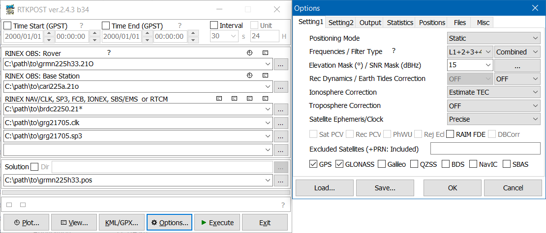
To use RTKLIB for RTK, install the latest version of RTKLIB (2.4.3 b34 or later), or Emlid RTKLIB QT (this is slightly outdated, and may crash with Garmin RINEX files). Note that on Windows, you need to install it into a folder that you have unrestricted write access to, as it stores settings files in that same folder (you will need to run it as an administrator if you put it in the C:\Program Files directory). Run rtkpost or rtkpost_qt. Under "RINEX OBS: Rover", select the RINEX output file you got from your device. Under "RINEX OBS: Base Station", select the RINEX file you got from the Ordnance Survey site. Under "RINEX NAV", select the ephemeris files (the unzipped files you got from the NASA site), on one line, using a wildcard ("*") to make it use more than one at a time if needed, eg. "C:\path\to\brdc1230.21*". In the inputs below that, you can optionally select the clk file and sp3 file (in separate inputs). Most inputs will allow you to use a wildcard ("*") to select multiple files, so that you can work with separate data files covering separate timespans (eg. one file per day). If using a "*.nav" file from a high quality device, select that instead of the "brdm*" or "brdc*" files.
Click "Options" and select the "Setting1" tab. Under "Positioning Mode", select "Static". Under "Frequencies / Filter Type", select "L1+2+3+4+5" (or "L1+L2+L5" in older releases) and "Combined" (this double Kalman filtering greatly improves the result accuracy when using a base station). For "Ionosphere correction", "OFF" is a good place to start, but test the options; "Estimate TEC" did very well for horizontal position, in personal testing. For "Troposphere correction", "OFF" is a good place to start, but test the options again; "Estimate ZTD" made the horizontal position a little worse and the height much worse, in personal testing. For "Satellite Ephemeris/Clock", select "Broadcast" to only use the brdm or brdc files, or "Precise" to also use the clk and sp3 files; "Precise" works better when Ionosphere correction is enabled, but in personal testing was worse than using "Broadcast". Enable all constellations and SBAS that are supported by both your GNSS device and the base station (OS Net only supports GPS and GLONASS), as well as the CLK and SP3 files if you are using them. Select the "Positions" tab. Under "Base Station", select "RINEX Header Position". Enable "Antenna type", leave it blank and set "Delta-E/N/U" to the phase centre offset northing easting and height for the base station (leave them at 0 if you don't know). Under "Rover" you can also do the same for the details of your GNSS device, so you do not have to manually subtract it later. Enable "Antenna type", leave it blank and set "Delta-E/N/U" to the phase centre offset northing easting and height for your GNSS device (eg. "0", "0", and "-0.033" for a Garmin GPSMAP 66sr). You can also upload data files for the antennae using the "Files" tab, as well as many of the other data files that Net_Diff uses to improve its results. In this case, you can set the antenna details to "*" to make it automatically use the correct antenna details from the file; it can then correct all the phase centre offset variances for all the different angles, rather than just an average.
Close options and select "Execute". You can now export it as GPX, KML, or view the output file to see the latitude, longitude and height. You can also plot the solution file (after clicking the "Plot" button, you may need to use the "File" menu to open the .pos file it created) to see how well it worked.
If you wanted to post-process using PPP in RTKLIB, do not select a "RINEX OBS: Base Station" file. Under "Options", select the "Settings1" tab. Under "Positioning Mode", select "PPP static". Under "Frequencies / Filter Type", select either "Forward" or "Backward". Enable all constellations and SBAS that are supported by your GNSS device, as well as the CLK and SP3 files if you are using them. On the "Positions" tab, do not set any offsets for the base station. The rest of the steps are the same as before. The results will be much better from a higher quality device, and from very long captures. Note that PPP Static mode seems to be broken in 2.4.3 b34 (it always returns empty results), while it works correctly in earlier versions.
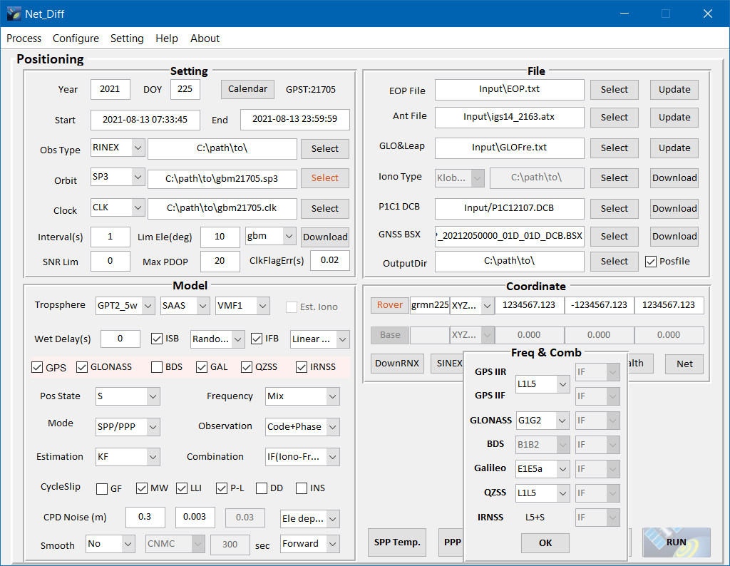
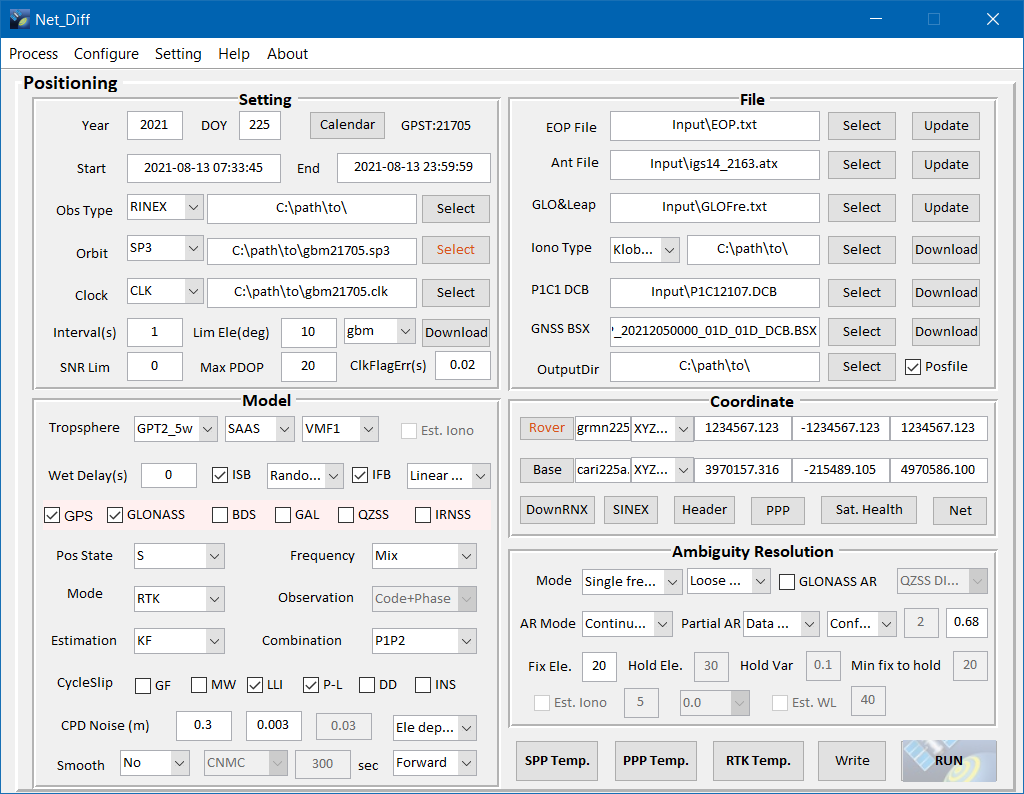
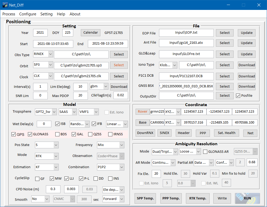
To use the Net_Diff desktop application for PPK or PPP, follow its instructions for installation (including utilities like gzip). Make sure you install it into a folder that you have unrestricted write access to, or you will need to run it as an administrator to avoid cryptic errors. If you run it from a Windows shortcut, make sure you set the working directory ("Start in") to the program's folder. Data files must be put into a folder without spaces in the path, such as C:\rinexfiles\.
Start Net_Diff. You can optionally use "Process - Download" to download relevant files like sp3 and clk. Select the year and date that readings were taken. Select an FTP server; IGN (igs.ign.fr) works well from Europe. Select the data files folder, and tick only the files you want (sp3 and clk are the main ones). Select an "AC" (analysis centre); some are better than others, but "igs" and "igr" are good for GPS only, "esa" is good for GPS or GLONASS, and "com" (Center for Orbit Determination in Europe) and "gbm" (GeoForschungsZentrum) are the best for GPS, GLONASS, Galileo, BeiDou and QZSS. "sha" covers GPS, GLONASS, Galileo and BeiDou, but uses a slightly outdated reference frame, though the results are still very good in the British Isles. Other sources may miss files, or have very few reference stations, or cover only a few satellites, or wait several minutes between measurements. If you don't know which one to use, select "gbm" or "com"; "gbm" has slightly better coverage of BeiDou satellites, and is the default analysis centre used by Net_Diff.
Use "Process - Positioning". Although it might be tempting to go through the options one by one, it is much better to set a few of the more important options first, so that it can helpfully fill in some of the other fields for you. Firstly, click on "Rover" and select your RINEX file. This will fill in the "Year", "DOY", "Start", "End", "Obs Type" and folder path, "Interval(s)" and "OutputDir", as well as the rover coordinates. Secondly, set the "Mode" to "SPP/PPP" or "RTK" (which is actually PPK), depending on which one you are trying to use. This will reset the "Wet Delay(s)", selected constellations, "Pos State", "Frequency", "Combination" and "CycleSlip" to defaults. So get it out of the way now to avoid it undoing your selections later. PPP and RTK modes need the device to record carrier phase information. SPP is like PPP without using carrier phase information. DSPP is like PPK without using carrier phase information. If your device cannot record useful carrier phase information, you can use one of those modes instead, but the results are very poor, so it is best not to use a device that cannot record useful carrier phase information. (DPPP is like a combination of PPP and PPK, which should refine PPK to a more precise point. However, in personal testing, it caused the results to slowly wander around without approaching the right position, so it is not recommended.)
Under "Setting", select the year and date that readings were taken (these should have been filled in for you, but use the calendar if not). "Obs Type" should be "RINEX". Beside it, select the folder where you put the data files (when using PPK, the base station file must also be in this folder). "Orbit" should be "SP3" (or you can use "broadcast" to select the less accurate "brdm*" or "brdc*" files, or the "*.nav" file from a high quality device). If you have already downloaded an sp3 file, select it using the button to the right, or the folder containing multiple files. If you have not downloaded it yet, select the folder where you want it to be downloaded to, such as the folder containing your data files. It will usually fill in the orbit file correctly when you select an sp3 file, but make sure. "Clock" should be "CLK" (or you can use "broadcast" to select the less accurate "brdm*" or "brdc*" files, or the "*.nav" file from a high quality device). If you have already downloaded a clk file, select it using the button to the right, or the folder containing multiple files. If you have not downloaded it yet, select the folder where you want it to be downloaded to. If you have not already downloaded the sp3 and clk files, select the right analysis centre in the box immediately below, such as "gbm" (this does not let you select an FTP service so if it fails you will need to use "Process - Download"), then click the "Download" button beside that. If the files do not appear in the folder(s), then they are not available yet, and you will need to wait for a while longer before trying again. Set "Interval(s)" to how often your device takes a reading (typically "1", but you can look for timestamps in the file to check).
Under "Model", set the "Wet Delay(s)" to either 0 or 7200 (or any non-zero value) for PPP, or 0 for PPK; 0 gave better results for PPP in personal testing. Select all constellations supported by your GNSS device for PPP (except IRNSS, which will never be used since it has no precise clock data), or both your device and the base station for PPK/DSPP/DPPP (eg. GPS and GLONASS only for OS Net). Set "Pos state" to "S" (static positioning), and "Frequency" to "Mix". Select the frequency sets your device supports, such as "L1L5" for GPS and QZSS with many devices, and close the subdialog. Now go back and set the "Pos state" again if it changed it (grrr). For SPP/PPP or DSPP/DPPP, set "Observation" to "Code+Phase" if your device can capture useful carrier phase information, or "Code" if not (test it and see which one works, results will be very poor without carrier phase tracking, as it has to use SPP or DSPP mode instead of PPP or DPPP). Set "Estimation" to "KF" (Kalman filtering). Set "Combination" to "IF(Iono-Free)" on a dual frequency device for PPP or "P1P2" on a dual frequency device for PPK (even if the base station data is single frequency), or "P1" on a single frequency device. With "CycleSlip", enable "LLI" and "P-L" (this helps with single frequency satellites, even in dual frequency operation), and for dual frequency operation, enable "MW" too. ("MW" also improved results with single frequency operation on a dual frequency device in personal testing, but Net_Diff displays a warning). Disable "GF", because it causes worse results when combined with others, in personal testing.
Under "File", click all three "Update" buttons (these files update very infrequently but there may be an update available). Set "Iono Type" to "None" (or leave it disabled) for PPP when using a dual frequency device, or "Klobuchar" and click the "Download" button on its line for PPK or single frequency PPP. Under "P1C1 DCB" click "Download". Do the same for "GNSS BSX". Select your desired "OutputDir". If using PPK or DSPP/DPPP, click on "Base" and select the base station file, then click "Header" to get its location. For PPK, set the "Mode" to whichever combination is possible; your GNSS device and the base station must support the same two frequencies for at least one satellite constellation to use "Dual/Triple", so select "Single freq 1" if not (this enables single frequency operation, even if the device or base station are dual frequency). You may need to re-select the sp3 and clk files/folders, because it sometimes unsets them (another bug). Click on "Run" and wait for it to finish processing.
If it immediately responds that it is done but no output files were created, something went wrong. Maybe it failed to download the Klobuchar data file (in which case you will have to set that to "None" and try again), or perhaps you selected the wrong files or options. If it created output files but there is no actual data after the commented header in the ".pos" file, then you probably selected the wrong number of frequencies for PPK, or your base station and device do not log compatible frequencies, or your device did not gather any carrier phase data; correct the options and try again. If it created output files but the results cut out after a very short time, your device probably had problems gathering carrier phase data (phones such as the Samsung Galaxy S10 lost carrier phase data after a few minutes in personal testing); try again with "Observation" set to "Code" for PPP, or use DSPP instead of PPK. Some poor data captures (eg. this happened in one test where the device stopped recording data for some satellites, and did not have enough left for a location fix) can also cause this issue with a non-zero "Wet Delay(s)", so try setting that to 0. In some cases you might have to email the author and ask what you did wrong.
When it finishes and asks if you want to see the results, say yes (this shows the same view that you can get to using "Process - Analysis"). At this point, you can optionally use the "Plot" button to get an idea of what the results look like, which can help with deciding how much data to ignore. Set the "Conver. Time(mins)" to the number of minutes of initial data that you want to ignore (60 is a good number) and click the "Make Report" button. When that finishes, open the report, and scroll down to the table to see the results. If you need to change settings and reprocess, you might need to close the app and start again, as it sometimes fails to recognise the changes correctly. If you need assistance with any of that, ask the author of the application for advice.
If you have a high quality GNSS antenna on your device, it is possible that Net_Diff will have already compensated for its antenna phase centre offset. With PPK, it is extremely likely that it will have already compensated for the phase centre offset of the base station since base stations tend to use common antennae. To check this, look in the report for the "Base Antenna Type" (for PPK) and "Rover Antenna Type" (for PPP or PPK). Open Net_Diff's antenna file; this is the file in the "Ant file" input, which is by default in <Net_Diff install directory>\Input\igs14_<number>.atx. Search for the first part of each antenna name, such as "LEIAR25". If you find a section for that antenna with either subtype "NONE" or the correct subtype, then Net_Diff has compensated for that antenna. If not, or if there was no antenna type for either of them in the report, then it will not have compensated for it. With a Garmin GPSMAP 66sr, the antenna type is left blank, so you will need to subtract -0.033 metres from the height of the results (ie. add 3.3 cm to the height) to get the tip of the antenna. With a high quality but relatively uncommon antenna such as an ArduSimple, Net_Diff might not know about it, but you can download the antenna calibration files from the manufacturer, and manually add its contents to the end of the main antenna file (this is needed with ArduSimple antennae, for example). When using an antenna which does not have any proper calibration data, there is likely to be a few centimetres of additional error in the vertical position, because Net_Diff cannot detect the difference between troposphere distortion, and the influence of the phase centre offsets for the different frequencies.
If you need to process a data file that covers more than one UTC day, then the process is a little more complicated. Firstly, set the "Year" and "DOY" to the first day. Set the "Orbit" path to an empty directory, and set the "Clock" to an empty directory. Use the "Download" button below the "Orbit" and "Clock" inputs to download them. Use the same approach with "Iono Type" and "GNSS BSX" inputs. Set the "GNSS BSX" input back to the folder path. Change the "Year" and "DOY" to the next day, and repeat the process. Once you are done with all the required days, set "Year" and "DOY" back to the first day. Set "End" to the end of the last day. Set the "GNSS BSX" input back to the folder path. PPP processing should now work. For PPK, the base station files need to be combined into a single file if they are separate.
You can also experiment with the other options, using the Guide To Using Net_Diff (see the product website) to work out what they mean. For example, you could try to enable "Wet Delay(s)" to estimate the troposphere parameter when using PPP. Check the standard deviation of the results to see if it is helping. You can also enable code smoothing using the "Smooth" input and "CNMC" for dual frequency or "P1" for single frequency. In personal testing, these made the results a little worse, with the wet delay causing the height error to increase. The "Forward" positioning type (the last input under "Model") can be changed to "Forward+Backward", which mimics the filtering setting in RTKLIB, but the results are much more challenging to interpret, so this option is not recommended; leave it on "Forward".
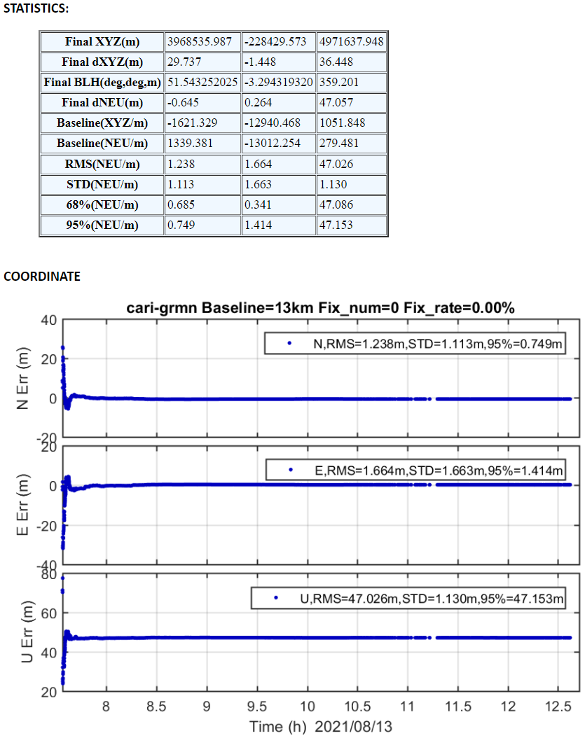
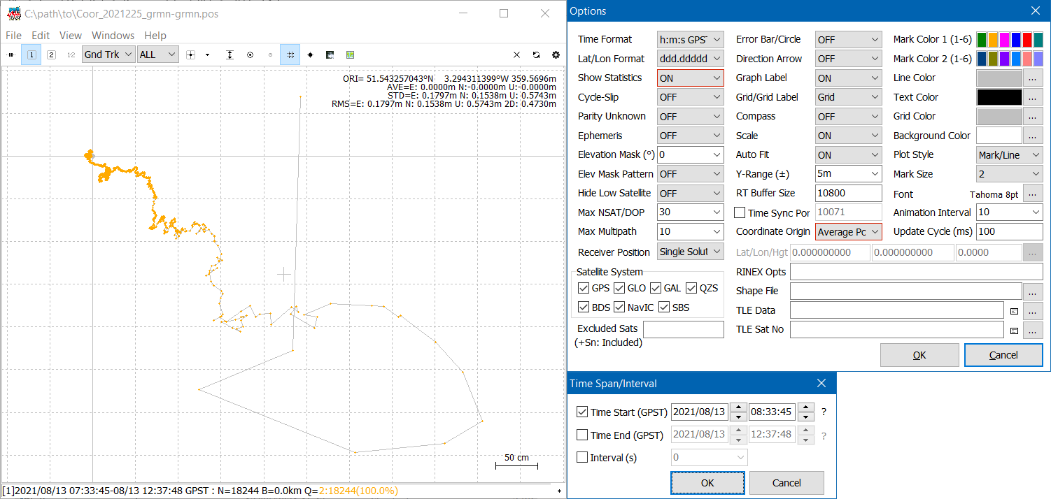
Post processing results are usually delivered in a ".pos" file. After some comment lines, the results are usually specified one line after another. Since you are looking for a single result, this may seem odd to have multiple results, but it is normal. Note that you may need to subtract 360 from the latitude if it is higher than 180, if you are manipulating the contents of the file manually.
The real art (or science) comes in working out how to interpret the results. With PPP the results are supposed to refine into a more and more perfect point, the last record in the file is the most refined one. With PPK and sometimes with PPP, they continue to rattle around, such that an average would be better, perhaps ignoring the initial part of the data which can be quite noisy. You may also see occasional results sitting far outside the expected area, depending on how well the Kalman filtering was applied - this happens a lot more with results from RTKLIB than Net_Diff. Such results should ideally be ignored as they may affect any averaging.
With RTKLIB, the final coordinates can be obtained using rtkplot; the view you get when you click on the "Plot" button after processing. To view the origin (resulting coordinates) and see the separate easting (longitude), northing (latitude), and height standard deviations, use "Edit - Options", and set "Show Statistics" to "ON". "Coordinate Origin" should normally be set to "End Pos" for PPP or "Average Pos" for PPK. (You can also choose to use "Linear Fit Pos", if you prefer that approach, but the resuts are generally less realistic.)
Net_Diff always shows the final position for "static" points in the report that it can prepare, and the standard deviations for northing (latitude), easting (longitude) and height are specified separately. Note that the results in that report may have different millimetre-level rounding errors compared with the .pos file. When calculating the standard deviations of PPP data, it ignores the initial subset of the data (by default the first 30 minutes, but 60 minutes is often better), as this is very inaccurate while it works out how to refine the position. It defaults to not ignoring any data with PPK, even though this also shows the same initial inaccuracy. In personal testing when using a phone antenna in a built up area with a partially obscured view of the sky, and a lot of reflections caused by buildings, the first 200 minutes needed to be ignored, because it took that long for the resulting data to converge. With data from a high quality antenna, ignoring 5 hours of initial data on captures of twice that length might leave only the tiniest residual jitter, when using PPK.
If you are trying to perform similar standard deviation calculations with RTKLIB, you may want to do something similar there; when viewing it in rtkplot, use "Edit - Time Span/Interval" to plot only the data after the first 30-60 minutes.
While RTKLIB's rtkplot makes it easy to see the average position, Net_Diff does not, but it is the best approach for PPK. To obtain this average, you can simply open the resulting .pos file in rtkplot. However if you would like to just use Net_Diff, open "Process - Analysis". Set the "Conver. Time(mins)" to the number of minutes of initial data that you want to ignore. Under "Coordinate - File1", select the resulting .pos file, and click on "Make Report" again. This will overwrite the HTML report file (make a backup first) using only the basic results. Open that file in your browser once processing completes. This will show the Mean BLH (latitude, longitude, height), which is the average.
Net_Diff calculates results to 1 mm precision in its reports, and can produce horizontal or vertical rounding errors of 1 mm on different computer hardware. This limitation is largely irrelevant unless you are trying to refine positions to greater than 1 mm precision (such as when setting up a fixed base station). However, Net_Diff's ".pos" file results are computed at 0.1 mm precision. If you want the results at that higher precision, then rather than asking Net_Diff to prepare a report, use rtkplot to process the ".pos" file.
When performing PPK with OS Net data, the results (including any KML files) will be in ETRS89 coordinates, not WGS84 (because that is what OS Net uses for the base station data). If you open a KML file in Google Earth, the results will be slightly displaced by the continental drift - that is expected. When performing PPP, the results will be in standard WGS84 GPS (actually since the recommended SP3 and CLK analysis centres use ITRF2014 as their reference frames, the coordinates will be in ITRF2014 current epoch, but as stated above, that is practically identical to WGS84, and it is what the HowToCreate tool uses). Remember to put them into the correct inputs when using the HowToCreate High Accuracy conversion tool.
There is a difficulty in knowing which options are working best for you. In general, if you want to know which method or option is performing best, you would need to compare it with a location that has been fixed extremely accurately. In personal testing, the results from Net_Diff with the suggested options were so accurate that when comparing with a landmark such as a trigpoint or benchmark, it was not possible to know if the small errors were caused by imperfections in the selection of post-processing options, or imperfections in the traditional surveying coordinates of the trigpoint or benchmark. As a result, the only reliable way to test it is by comparing with the results from a true differential (NRTK or RTPPP) GNSS device. If you have access to one of those for testing, you should really be using that for surveying instead.
However, without a more accurate device to test against, you can try two separate captures from the same location on different days and see if those are nearly the same; this tests for randomness in positioning. You can try rotating the device horizontally so that the antenna is still in the same position but the device is now facing in the opposite direction or 90° away, and see if it still records the same position in each case; this can help test for biases in the device's antenna. You could try moving it to each corner of a measured 5 metre square to take more readings, and see if the square ends up being 5 metres when the results are plotted; this helps test for biases caused by reflections if you test it in a city garden. You can also try different options, and see if the standard deviation of the results gets better or worse; this helps to work out if an option is likely to be causing the results to improve. Of course, these don't help you detect if the options you have chosen are actually good; if the results are consistently bad (eg. if an option causes the result to always be shifted 20 cm eastwards), you would not be able to tell without a proper fixed location. And before you ask; the Ordnance Survey are highly unlikely to let you stand next to their OS Net antennae to test your device. You can of course rest happy in the knowledge that if you have managed to fix the location of a trigpoint well enough that you cannot tell if the errors are in your own post processing of the data, or the Ordnance Survey's traditional surveying of the trigpoint, then your location fixing is easily good enough to be used for fixing a cave survey.